Periodogram and spectral density: Definition & Examples

A spectral density allocates a stationary time series' variance across frequencies. A periodogram estimates that frequency distribution from a finite sample by squaring and scaling its Fourier coefficients. For a quant studying returns, order flow or a model's residuals, this can reveal whether variation concentrates at slow or fast timescales. A tall peak alone does not establish a stable trading cycle.

The distinction is between a property of the stochastic process and a noisy statistic computed from observations. It is also a distinction between density and power: a density height must be multiplied by a frequency width before it becomes a contribution to variance.

The process has a spectrum; the sample has a periodogram

Let

x_t

be a real-valued, weakly stationary process with mean

\mu

and autocovariance

\gamma(h)=\text{Cov}(x_t,x_{t+h})

. Suppose

\sum_h\lvert\gamma(h)\rvert<\infty

. With frequency

\nu

in cycles per sample, its two-sided spectral density is

S(\nu)=\sum_{h=-\infty}^{\infty}\gamma(h)e^{-2\pi i\nu h}, \qquad -\tfrac12\leq\nu\leq\tfrac12, \qquad \gamma(0)=\int_{-1/2}^{1/2}S(\nu)\,d\nu.

This is the Fourier transform of the covariance sequence, not the probability density of a return. Its area is variance, not one. Larger low-frequency density means more variance associated with slow variation. Bartlett's spectral-density notes give this transform and inverse relationship. The summability assumption is sufficient for this ordinary density representation; stationary processes with spectral lines require a more general spectral measure.

If samples arrive at rate $f_s$ per time unit, physical frequency is $f=f_s\nu$ and density rescales as $S_f(f)=S(f/f_s)/f_s$ . Integration over $[-f_s/2,f_s/2]$ still gives the same variance. Cycles per day, cycles per observation and radians per observation are different conventions.

Follow the units through the FFT

For $N$ equally spaced observations, let $y_t=x_t-\bar x$ when removing the sample mean is appropriate. Use the unnormalised discrete Fourier transform:

X_k=\sum_{t=0}^{N-1}y_t e^{-2\pi i kt/N}, \qquad \Delta f=\frac{f_s}{N}, \qquad I_2(f_k)=\frac{\lvert X_k\rvert^2}{f_sN}.

An FFT is an efficient algorithm for this DFT; it does not choose the statistical interpretation or scaling. The bins above the positive Nyquist limit represent negative frequencies: for even $N$ , $k>N/2$ maps to $(k-N)f_s/N$ .

For real observations, positive and negative interior frequencies carry equal power. A one-sided density keeps

0\leq f\leq f_s/2

and doubles the interior positive ordinates. Do not double DC (

k=0

) or, for even

N

, the Nyquist bin (

k=N/2

). For odd

N

there is no Nyquist bin, so every retained positive bin is doubled. Complex-valued data generally need the two-sided representation. SciPy's periodogram reference documents its one-sided folding and scaling choices.

The density units are amplitude squared per unit of frequency. With this rectangular window and no zero-padding,

\sum_k I_2(f_k)\Delta f =\sum_{k\geq0}I_1(f_k)\Delta f =\frac1N\sum_{t=0}^{N-1}y_t^2.

This is the finite-sample Parseval audit. After demeaning, the right side is the sample variance with denominator $N$ , not the unbiased $N-1$ estimator. Without demeaning, it is the raw mean square and includes the mean's DC contribution.

Eight constructed observations

Take the dimensionless deterministic signal

x_t=\cos(2\pi\cdot2t/8),\quad t=0,\ldots,7,\qquad f_s=1.

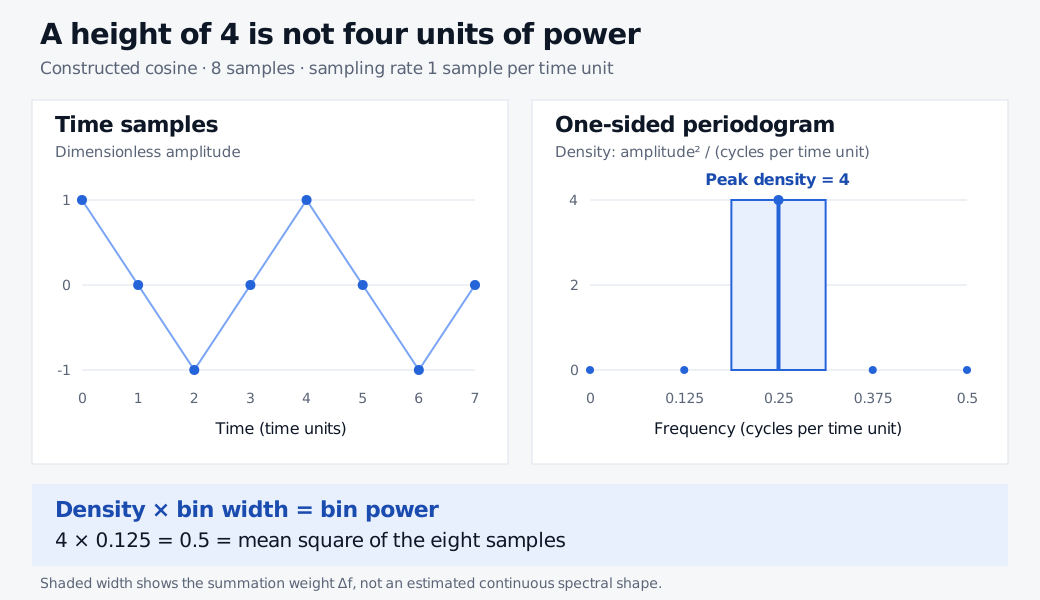
Its values, ignoring numerical rounding, are $1,0,-1,0,1,0,-1,0$ . The mean is zero. It completes two cycles in the eight-sample record, with period four time units. Only $k=2$ and $k=6$ have nonzero DFT magnitudes: both equal four.

Quantity	Calculation	Result
Raw squared coefficient at $k=2$	$\lvert X_2\rvert^2$	$16$
Two-sided density at $f=0.25$	$16/(1\cdot8)$	$2$
Matching negative-frequency density	$I_2(-0.25)$	$2$
One-sided density at $f=0.25$	$2+2$	$4$
Frequency bin width	$1/8$	$0.125$
One-sided bin power	$4\cdot0.125$	$0.5$
Sample mean square	$(1+1+1+1)/8$	$0.5$

Constructed eight-point cosine has mean square 0.5. Its one-sided periodogram has density 4 at 0.25 cycles per time unit; multiplying by bin width 0.125 gives power 0.5.

Original deterministic illustration. The shaded width represents the frequency summation weight, not a continuous population spectral curve.

If the same eight values are instead sampled at $f_s=2$ , the positive peak moves to $0.5$ cycles per time unit, its density becomes $2$ , and bin width becomes $0.25$ . Power remains $2\cdot0.25=0.5$ . Neither the value four nor the eight observations prove a stochastic market cycle; this example isolates the bookkeeping.

INTERACTIVE EXPLORER

Finite Fourier spectrum

Sample two sinusoids and inspect aliasing, leakage and bin power.

Two reasons a real curve is harder to read

Finite observation spreads power. A sinusoid between Fourier bins leaks into nearby bins. A taper such as Hann reduces distant sidelobes while broadening the main lobe, making nearby components harder to separate. Zero-padding evaluates a denser frequency grid; it supplies no additional observations. The SciPy spectral-analysis guide illustrates these effects.

A density-scaled tapered periodogram uses

I_{w,2}(f_k)=\frac{\left\lvert\sum_t w_ty_te^{-2\pi i kt/N}\right\rvert^2} {f_s\sum_t w_t^2}.

Its integrated ordinate sum equals $\sum_t w_t^2y_t^2/\sum_t w_t^2$ , which need not equal the unweighted mean square. Amplitude calibration uses a different normalisation. Record the actual taper and mean/trend treatment; changing either changes the object being measured.

More data do not make each raw ordinate settle down. Under standard short-memory conditions, the unsmoothed periodogram is not a consistent estimator of the spectral density at an interior frequency with positive density. In the Gaussian white-noise case, at a nonzero, non-Nyquist Fourier bin with

f_s=1

\frac{2I_2}{\sigma^2}\sim\chi^2_2, \qquad \mathbb E[I_2]=\sigma^2, \qquad \text{Var}(I_2)=\sigma^4.

That variance does not shrink as

N

grows. Bartlett's periodogram lecture develops the exact white-noise result and the asymptotic argument. Smoothing nearby frequencies can trade detail for stability. Welch's method averages tapered segment periodograms; shorter segments sacrifice frequency resolution, and overlapping segments do not supply independent replications.

Before calling a peak economic evidence

Justify the sampled clock and transformation. Irregular trades cannot simply be treated as equally spaced calendar-time data. Variation above the Nyquist frequency can alias into lower frequencies. Changing regimes, a trend or deterministic intraday seasonality can dominate the picture. Mean removal alone does not establish stationarity; the Stationarity and Unit Roots lesson distinguishes stationary fluctuations from unit-root levels and deterministic trends. Its public page is a preview; the full lesson requires membership.

Report the sample interval, units, detrending, taper, FFT length, side convention and smoothing rule. Then assess uncertainty, frequency-search effects and stability on new data before interpreting a peak as a repeatable mechanism. For comparing frequency-specific relationships between two series, cross-spectrum and coherence add joint phase and association; two auto-periodogram peaks alone do not show a shared stable relationship.

Sources

Peter Bartlett, Introduction to Time Series Analysis, Lecture 19, slide 2: population spectral density and covariance inversion.
Peter Bartlett, Lecture 20, slides 3–8 and 11–19: periodogram normalisation, Parseval identity and inconsistency.
SciPy, periodogram reference: sampling frequency, one-sided folding and density versus spectrum scaling.
SciPy, Spectral Analysis: finite records, leakage, taper normalisation and zero-padding.
SciPy, welch reference: averaging segment periodograms and estimator settings.