Cross-spectrum and coherence: Definition & Examples

The cross-spectrum describes how two time series vary together at each frequency, retaining both the size and relative phase of their joint oscillations. Magnitude-squared coherence normalises that cross-spectrum by the series' individual spectral power, producing a frequency-specific measure of linear association between zero and one. For a quant comparing return signals, it separates shared slow variation from shared fast variation that a single contemporaneous correlation can conceal.

High coherence does not establish causation, a forecast available in real time, or a profitable lead–lag trade. It describes a second-order relationship at a frequency.

Fix the convention before reading the phase

Consider real-valued, equally spaced, jointly weakly stationary processes $x_t,y_t$ . Define the cross-covariance in this article as

\gamma_{xy}(h)=\text{Cov}(x_t,y_{t+h}).

When the covariance sequences are absolutely summable, their Fourier transforms give spectral densities. Our cross-spectrum is

S_{xy}(f)=\sum_{h=-\infty}^{\infty}\gamma_{xy}(h)e^{-2\pi i f h}, \qquad -\tfrac12\leq f\leq\tfrac12.

Here

f

is in cycles per sample, rather than radians per sample. The corresponding auto-spectra

S_{xx},S_{yy}

describe each series' variance by frequency; for example,

\text{Var}(x_t)=\int_{-1/2}^{1/2}S_{xx}(f)\,df

. The cross-spectrum can be complex even though the observations are real.

With the negative-exponent discrete Fourier transform, this definition corresponds to conjugating the first transform:

\overline X Y

. Reversing the series order conjugates the cross-spectrum, changing the phase sign while preserving its magnitude. Some references use the opposite cross-covariance indexing and hence the opposite sign. SciPy's csd(x, y) uses the convention chosen here. SciPy documents this explicitly.

For a positive-gain pure delay $y_t=a x_{t-\tau}$ , $a>0$ , the cross-spectrum's phase is $\phi(f)=-2\pi f\tau$ modulo $2\pi$ . Thus a negative phase at a positive frequency is consistent with $y$ lagging $x$ under this delay model. A general filter need not correspond to a single delay. Phase is undefined when the cross-spectrum is zero and unstable when it is poorly estimated.

Three quantities that should stay separate

The complex coherency, its magnitude, and its squared magnitude are different objects:

K_{xy}(f)=\frac{S_{xy}(f)}{\sqrt{S_{xx}(f)S_{yy}(f)}}, \qquad C_{xy}(f)=\lvert K_{xy}(f)\rvert^2 =\frac{\lvert S_{xy}(f)\rvert^2}{S_{xx}(f)S_{yy}(f)}.

We call $C_{xy}$ magnitude-squared coherence throughout. It is dimensionless and lies in $0,1]$ where both auto-spectra are positive; it is undefined if the denominator is zero. The bound follows from the positive semidefinite spectral matrix, equivalently a frequency-domain [Cauchy–Schwarz inequality.

Coherence measures linear association with a stable relative phase, not whether the two individual spectra merely peak at the same frequency. It also discards direction and sign: a stable negative relationship or delay can have coherence one. Zero coherence does not exclude nonlinear dependence. The Berkeley notes relate squared coherence to the variance accounted for by a linear filter; that filter may use future observations, so the interpretation does not automatically deliver a usable forecast.

Why a raw FFT ratio tells you nothing

For one length- $N$ rectangular segment, use the unnormalised DFT

X_k=\sum_{t=0}^{N-1}x_t e^{-2\pi i kt/N}, \qquad I_{xy,k}=\frac{\overline{X_k}Y_k}{N}, \qquad I_{xx,k}=\frac{\lvert X_k\rvert^2}{N}.

These are two-sided periodogram ordinates at $f_k=k/N$ with sampling frequency one. Define $I_{yy,k}$ analogously. Whenever both transforms are nonzero,

\frac{\lvert I_{xy,k}\rvert^2}{I_{xx,k}I_{yy,k}}=1.

This is an algebraic identity for any pair of nonzero complex coefficients. It is not evidence of perfect population coherence. Estimate the spectra through averaging or smoothing first, then form their ratio. Welch estimation averages segment cross-periodograms and auto-periodograms; multitaper and frequency smoothing provide other approaches. The complex cross-values must be averaged before taking their squared magnitude. Gille's lecture demonstrates the order-of-operations issue.

Two fictional segments, one revealing cancellation

Take $N=24$ , $t=0,\ldots,23$ , and the dimensionless deterministic sequences

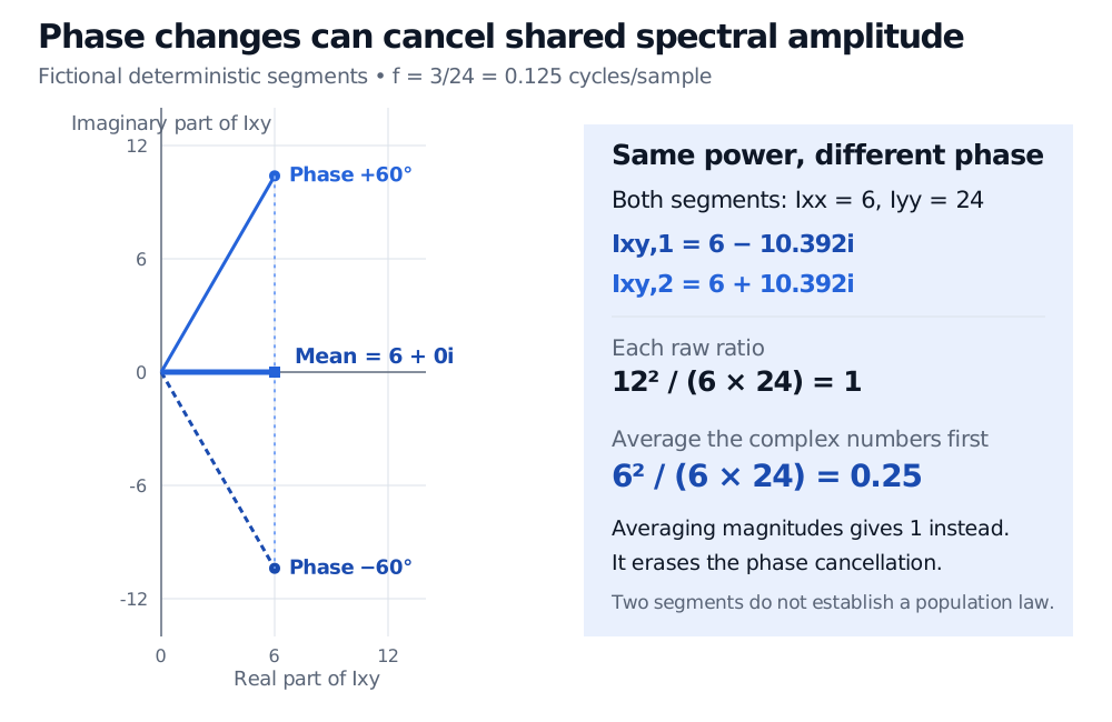
x_t=\cos(2\pi\cdot3t/24),\qquad y_t^{(-)}=2\cos(2\pi\cdot3t/24-\pi/3),\qquad y_t^{(+)}=2\cos(2\pi\cdot3t/24+\pi/3).

Each pair uses the same $x$ . At $k=3$ , $f=0.125$ cycles per sample, the period is eight samples. Both segments give $I_{xx}=6$ and $I_{yy}=24$ , but their cross-values differ:

I_{xy}^{(-)}=6-6\sqrt3\,i,\qquad I_{xy}^{(+)}=6+6\sqrt3\,i.

Each cross-value has magnitude 12, so each raw ratio equals

144/(6\cdot24)=1

. Average the complex values with equal weights instead:

\widehat S_{xy}=6,\qquad \widehat S_{xx}=6,\qquad \widehat S_{yy}=24,\qquad \widehat C_{xy}=\frac{6^2}{6\cdot24}=0.25.

Averaging magnitudes first would preserve 12 and incorrectly return one. The opposite phases cancel the imaginary components; this loss of phase consistency lowers the averaged statistic despite unchanged auto-power.

Two fictional 24-point segments at 0.125 cycles per sample have cross-periodograms 6 minus 10.392i and 6 plus 10.392i. Their mean is 6, giving magnitude-squared coherence 0.25 although each raw ratio equals 1.

Original deterministic illustration, dimensionless inputs and two-sided periodograms. Complex values are averaged before their magnitude is squared; the two segments illustrate arithmetic, not a population estimate.

For the minus-phase sinusoid alone,

\phi=-\pi/3

gives a delay

-\phi/(2\pi f)=4/3

samples, modulo the eight-sample period. This fractional shift describes the underlying sinusoid; it is not an observed execution delay or a uniquely identified lag.

What to report with an estimated curve

Specify the sampling interval, alignment, transformations, segment length, taper, overlap, detrending and averaging rule. In financial data, asynchronous observations and changing regimes can produce misleading phase or coherence. Joint stationarity needs justification; simply feeding two trending price levels into an FFT does not supply it. The Stationarity and Unit Roots lesson develops that prerequisite; its public page is a preview and the full lesson requires membership.

Use matching spectral conventions throughout. For real data, the usual one-sided density convention doubles interior positive-frequency ordinates of all three spectra; these factors cancel in coherence. Do not mix one-sided auto-spectra with an undoubled cross-spectrum. Taper normalisation and a different sampling frequency also change density units and values. SciPy's coherence documentation defines the estimator through matching spectral estimates.

Finally, uncertainty depends on the estimator and effective independent information. Overlapping segments are dependent, smoothing trades frequency detail for stability, and searching many frequencies changes the inference problem. The two deterministic segments above supply no confidence interval or independent-replicate population argument. A coherence peak needs an estimation and validation design before a researcher can interpret its economic significance.

Sources

Peter Bartlett, Introduction to Time Series Analysis, Lecture 25, slides 7–10 and 14–16: cross-spectra, smoothed estimation and linear-filter interpretation. Its cross-spectrum indexing conjugates our convention.
Sarah Gille, SIOC 221A, Lecture 17, pp. 1–4: conjugate-first cross-spectrum, phase under delays and complex averaging before magnitude.
SciPy, csd reference: transform order, scaling and Welch estimation.
SciPy, coherence reference: magnitude-squared coherence formula and estimation parameters.