Compare observed time-series statistics with null-consistent surrogate data, audit phase-randomisation constraints, and interpret finite Monte Carlo rank p-values.
Surrogate data testing
Surrogate data testing compares a statistic from an observed time series with the same statistic from artificial series generated under a specified null hypothesis. The surrogates retain properties that the null is meant to explain while randomising other structure. For a quant researcher, the question is whether an apparent signal needs an explanation beyond, for example, the series’ existing linear dependence. The null, generator and statistic must answer the same question. This is the framework introduced by Theiler and coauthors (1992).
A surrogate here is a null-data realisation, rather than an approximation to an expensive pricing function.
What gets to survive the randomisation?
Consider a strategy that appears to exploit the ordering of returns. Shuffling every return preserves the observed values but destroys serial dependence. Such a permutation test can ask whether temporal ordering matters under an exchangeable-data null. It cannot isolate nonlinear structure beyond a linear dependence pattern that the shuffle has also removed.
A Fourier phase surrogate offers a different comparison: keep the finite sample’s Fourier magnitudes and change its phases. This preserves the periodogram. A statistic sensitive to time asymmetry or nonlinear prediction can then examine structure outside those fixed second-order constraints. The choice of statistic, including its direction and tuning, belongs before inspection of the test result. Schreiber and Schmitz explain why different surrogate constraints represent different hypotheses.
An exact preservation check on sixteen fictional observations
Take an equally spaced, dimensionless sequence with these values in time order:
Replace the phases of bins k=1,…,7 with independent draws ϕk uniform on [0,2π):
Yk=∣Xk∣eiϕk,Y16−k=Yk.
Keep Y0=X0 and Y8=X8. The conjugate pairing makes the inverse transform real. The DC coefficient fixes the mean; the even-length Nyquist coefficient is real and is kept unchanged here. Neither can receive an arbitrary complex phase. For odd record length there is no Nyquist bin.
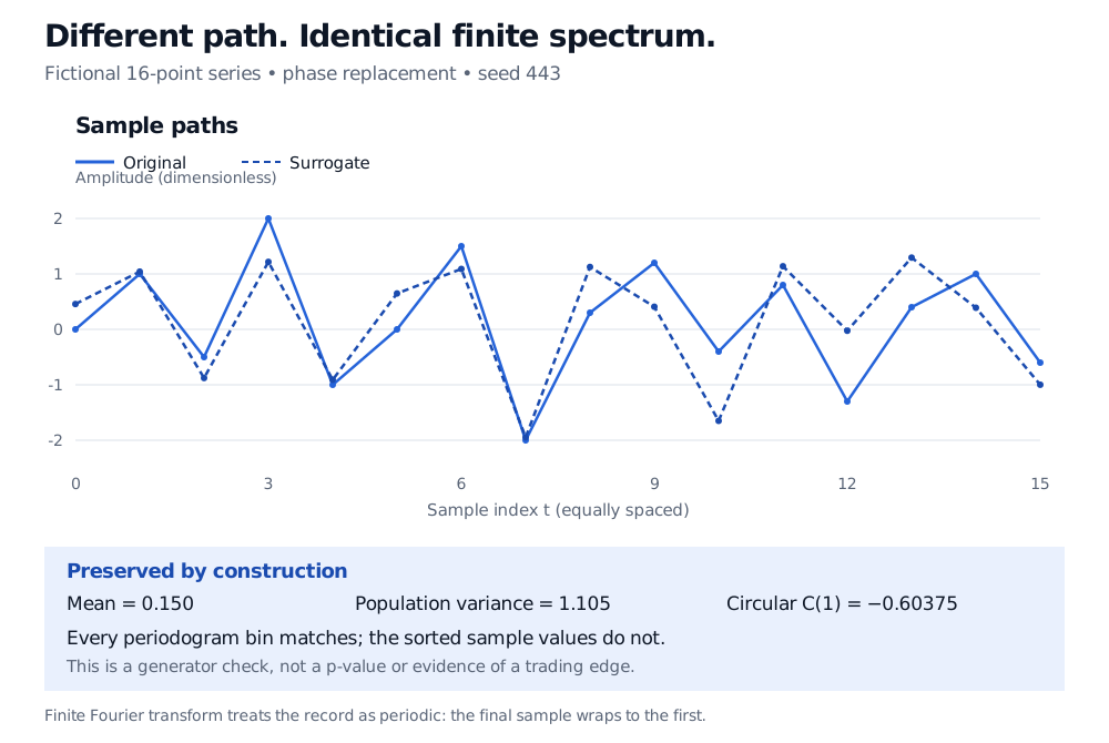
Using NumPy’s default random generator with seed 443 for the seven replacement phases produces a surrogate beginning 0.456891,1.040931,−0.876918,1.216869. These are new values, rather than a permutation of the original observations.
Original fictional 16-point series and seed-443 phase surrogate follow different paths. Both have mean 0.150, population variance 1.105 and circular lag-one covariance minus 0.60375; their periodograms match but their sorted values differ.
Original fictional example. Solid and dashed paths differ while the specified finite Fourier constraints agree to numerical precision.
The invariants follow directly from the construction. At unit sampling frequency, define the two-sided periodogram as Ik=∣Xk∣2/16. Every Ik is unchanged. In particular,
The denominator is 16: this is the population-form variance of each finite record. Fourier inversion of the squared magnitudes also preserves the circular sample autocovariance
Ch=161t=0∑15(xt−xˉ)(x(t+h)mod16−xˉ).
For both paths, C1=−0.60375. The wrap from the last observation to the first is essential. The ordinary truncated sample autocovariance need not match.
Consequently, testing this very circular autocorrelation function against these surrogates is uninformative: it was fixed by design. The amplitude distribution and nonlinear relationships were not fixed. In financial applications, preserving return autocorrelation does not preserve volatility clustering.
A rank calculation is a separate step
For an upper-tail test, let larger T mean stronger evidence against the null. With B surrogate statistics, a common finite Monte Carlo rank p-value is
p=B+11+∑b=1B1{Tb≥Tobs}.
Separate fictional illustration: suppose Tobs=3.2 and nine surrogate statistics are 0.2, 0.5, 0.8, 1.1, 1.4, 1.7, 2.0, 2.3 and 3.5. One is at least 3.2, giving p=(1+1)/(9+1)=0.20. These stipulated statistics were not computed from the sixteen-point FFT example. With nine surrogates, this convention cannot produce a p-value below 0.10.
The rank argument requires the observed and surrogate statistics to be exchangeable under the null. With no ties, each of the ten ranks is equally likely; counting ties with ≥ gives a conservative rule under exchangeability. The plus-one calculation does not repair a wrong generator. Phipson and Smyth, §4 derive the Monte Carlo correction.
For the generator above, one precise conditional null makes the observed interior Fourier phases independent uniform variables given the fixed magnitudes, DC and Nyquist coefficients. Under that null, replacing the phases yields the required conditional comparison. Merely describing a finite financial sample as a stationary Gaussian linear process does not automatically establish this exact phase law. Boundary effects, parameter estimation and approximation error require model-specific justification or calibration.
What the conclusion can support
Fourier surrogates treat the finite record as periodic. Endpoint mismatch, changing volatility regimes and other failures of stationarity can therefore drive rejection. Iterative amplitude-adjusted Fourier transform (IAAFT) methods alternate distribution matching and spectrum matching; finite outputs need an audit of the remaining mismatch, rather than a promise that both constraints are exact. These limitations are discussed in Schreiber and Schmitz, §§4.3–4.5 and 7.
For strategy validation, a result concerns the stated null and statistic. It does not by itself establish chaos, a causal mechanism or future net profitability. If strategy selection is part of the claim, the surrogate experiment must account for that selection; testing only a winning configuration understates the search. Likewise, shuffling fitted residuals needs a defensible residual exchangeability assumption. It is not a universal substitute for a financial time-series null.
For background on deciding which series can plausibly support a stable dependence model, read Stationarity and Unit Roots (public preview; full lesson requires membership). It distinguishes stationary fluctuations, unit-root levels and deterministic trends before a surrogate comparison is designed.