Summation notation: Definition & Examples

Summation notation uses the capital Greek sigma,

\sum

, to mean “add the specified terms.” In a portfolio formula it can compress hundreds of asset contributions into one expression, while making clear which assets belong in the calculation.

For integers $m\le n$ ,

\sum_{i=m}^{n} x_i=x_m+x_{m+1}+\cdots+x_n.

The index

i

tells you which term to use;

m

and

n

are the lower and upper bounds, both included. The summand

x_i

is the expression evaluated at each index. Here there are

n-m+1

terms. A subscript identifies a term; it does not mean multiplication by

i

Read the instruction before calculating

For example,

\sum_{i=2}^{4} i=2+3+4=9.

Starting at 2 gives three terms, not four. The index is a dummy index: renaming it consistently changes nothing, so

\sum_{i=2}^{4}x_i=\sum_{k=2}^{4}x_k

. Changing only the subscript or only the bound does change the instruction.

A sum may also specify a set, as in $\sum_{i\in A}x_i$ , meaning one term for every index in $A$ . A bare $\sum_i$ needs its index set supplied by context. The standard empty-sum convention gives zero when there are no indices to include. An upper bound of infinity needs an additional convergence argument; finite-sum algebra alone does not justify manipulating an infinite series.

Three assets, one portfolio return

Suppose initial portfolio weights are 50%, 30% and 20%, and the assets' assumed expected returns over the same single period are 8%, 4% and 1%. We use simple returns, fixed initial weights and no external cash flows, fees or trading during the period. These are synthetic inputs.

Let $w_i$ be the weight of asset $i$ and $\mu_i$ its expected return, written as a decimal. Then

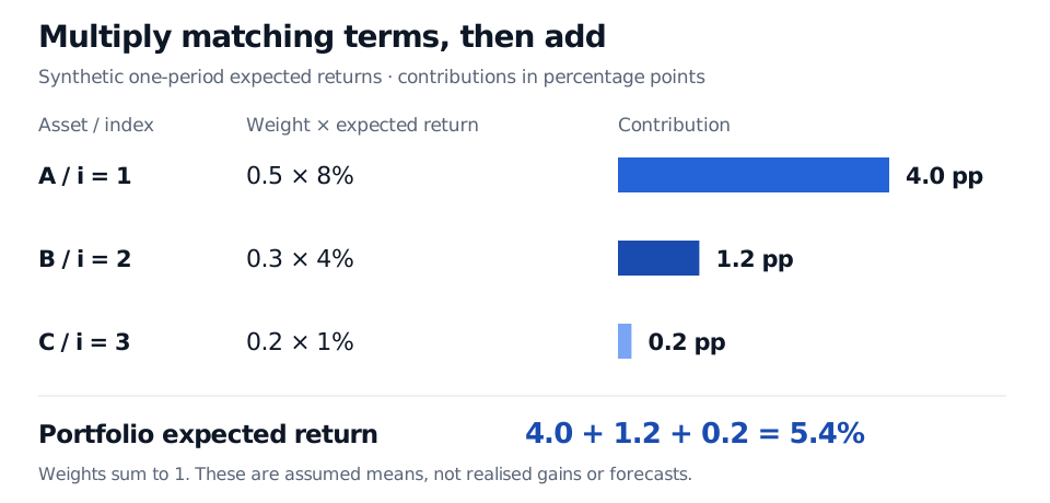
\mu_p=\sum_{i=1}^{3}w_i\mu_i =0.5(0.08)+0.3(0.04)+0.2(0.01) =0.054=5.4\%.

Three synthetic assets have weights 0.5, 0.3 and 0.2 and expected returns 8%, 4% and 1%. Their expected-return contributions are 4.0, 1.2 and 0.2 percentage points, adding to 5.4%.

Multiply each asset's weight by its own expected return, then add the contributions. All inputs refer to the same period; the result is an assumed portfolio mean.

The multiplication happens inside the sum. With initial wealth USD 10,000, the allocations are USD 5,000, USD 3,000 and USD 2,000; their expected profits are USD 400, USD 120 and USD 20. The total USD 540 divided by USD 10,000 gives the same 5.4%. This is an expectation, not a promised gain.

Weights are dimensionless, so multiplying a weight by a return leaves return units. In percentage notation the contributions are 4.0, 1.2 and 0.2 percentage points. Do not mix 0.08 for one return and 4 for another, or combine monthly and annual returns in the same calculation.

A sum is not automatically an average

The unweighted arithmetic mean is $\frac{1}{n}\sum_{i=1}^{n}x_i$ . A weighted mean with non-negative weights is

\frac{\sum_{i=1}^{n}a_i x_i}{\sum_{i=1}^{n}a_i}, \qquad \sum_{i=1}^{n}a_i>0.

Our portfolio weights already sum to one, so no further division is needed. Dividing its 5.4% weighted sum by three would count the averaging twice. Conversely, the unweighted mean of the three asset means is about 4.33%, which describes equal asset weights rather than this portfolio. With short positions, a weighted sum can still describe portfolio return under the stated financing convention, but it need not behave like an average bounded by the smallest and largest asset return.

What can move outside the sigma?

For constants $a$ and $b$ that do not depend on $i$ , finite sums satisfy

\sum_{i=1}^{n}(a x_i+b y_i) =a\sum_{i=1}^{n}x_i+b\sum_{i=1}^{n}y_i.

A common multiplier can move outside; asset-specific $w_i$ cannot. A constant summand is counted once per index: $\sum_{i=1}^{n}c=nc$ , not $c$ . Parentheses also matter: adding $c$ after the completed sum adds it once, whereas $\sum_{i=1}^{n}(x_i+c)$ adds it $n$ times.

For fixed portfolio weights and random returns with finite absolute expectations, linearity of expectation gives

\mathbb{E}\left[\sum_{i=1}^{n}w_iR_i\right] =\sum_{i=1}^{n}w_i\mathbb{E}[R_i].

Independence is not required. Assets may move together and still have their expected contributions add this way. Dependence matters for portfolio variance, which is a different calculation. If weights themselves are random and related to returns, replacing

\mathbb{E}[w_iR_i]

by a product of expectations needs additional justification.

For the probability-weighted sums behind this last identity, continue with Expectation, Variance and Covariance. The public page provides a preview; the full lesson is free with a signed-in account.

Sources

James Stewart, Single Variable Calculus: Early Transcendentals, 6th edition (2008), Appendix E, “Sigma Notation,” pp. A34–A35.
Dimitri P. Bertsekas and John N. Tsitsiklis, Introduction to Probability, 2nd edition (2008), §2.5, “Joint PMFs of Multiple Random Variables,” especially pp. 94–97.
James Aspnes, Yale University, Summation notation, §§1.1–1.5 and 2.2.
Columbia University, Summation Notation.

Read the instruction before calculating

Three assets, one portfolio return

A sum is not automatically an average

What can move outside the sigma?

Sources

Related terms

Expected return

Expected value

Portfolio variance