SWA averages late-training weights into one network; SWAG adds a local Gaussian weight approximation. Learn why neither is simply prediction averaging.
Stochastic weight averaging and SWAG
Stochastic weight averaging (SWA) takes an equal average of selected late-training parameter vectors to produce one neural network. SWA-Gaussian (SWAG) adds a Gaussian approximation over weights and averages predictions from sampled networks. For a quant fitting a financial forecasting model, these are different deployment choices: one fitted predictor versus a distribution of predictors whose uncertainty still needs evaluation.
What gets averaged?
Let w1,…,wT denote collected parameter vectors. SWA uses
wˉT=T1t=1∑Twt.
Here “weights” means model parameters, not portfolio allocations. A running implementation needs only the current average and a snapshot count:
wˉT+1=wˉT+T+1wT+1−wˉT.
The original method continues stochastic gradient descent from a trained model with a constant or cyclical learning-rate schedule. It averages points along that trajectory. The motivation is to move toward the interior of a broad region of good solutions, rather than stop at one visited point. The reported generalisation gains in Izmailov and coauthors' paper are empirical; they do not establish gains on financial data.
Averaging arbitrary independently trained networks is a different operation. Hidden units can be permuted without changing a network's function, while coordinate-by-coordinate averages of differently aligned units can damage it. SWA's trajectory construction matters; averaging is not automatically safe merely because individual models perform well.
Average first, or predict first?
Consider an original synthetic scalar predictor at a fixed input:
fw(x)=w2.
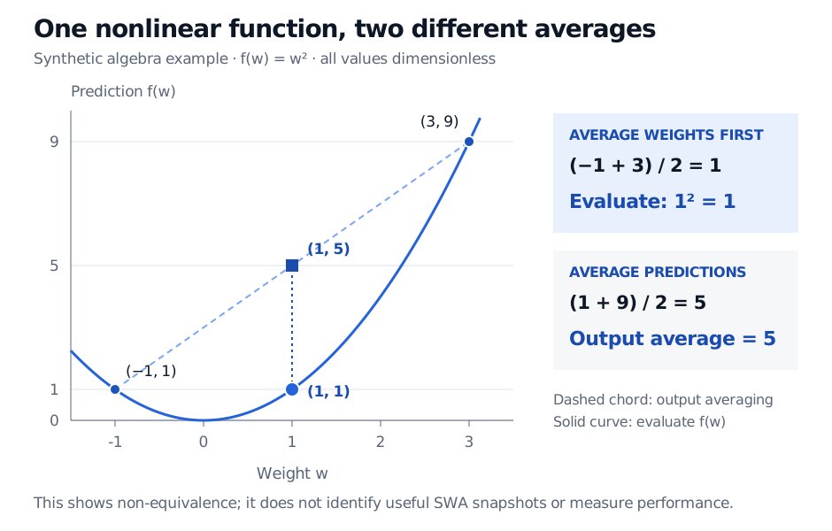
The input is held fixed, and all numbers are dimensionless. Stipulate two snapshots, w1=−1 and w2=3. Averaging their weights gives
wˉ=2−1+3=1,fwˉ(x)=1.
Averaging their predictions instead gives
2f−1(x)+f3(x)=21+9=5.
Synthetic predictor f(w) equals w squared. Snapshots minus one and three give outputs one and nine. Their average weight is one, whose output is one; the average of the two outputs is five.
Original dimensionless example. The chord midpoint averages outputs; the point on the curve evaluates the averaged weight. This is an algebra comparison, not a fitted loss landscape or evidence that these snapshots should be combined.
The difference comes from nonlinearity. Here the output average exceeds the output at the average weight by 4, exactly the population variance of the two equally weighted snapshots. For a function linear in its parameters, the two averages agree; a deep network generally lacks that property.
These snapshots were chosen to expose the arithmetic. They are not a simulated training trajectory, posterior samples or a recommendation to average separated modes. No target or loss was specified, so neither output can be called more accurate.
What SWAG adds
SWAG fits a local approximate weight distribution centred at the SWA mean. Its diagonal part uses coordinatewise second moments. Full SWAG supplements this with a low-rank term capturing directions of joint movement along the training trajectory. In the original paper's construction,
q(w)=N(wˉ,21[Σdiag+K−1DD⊤]).
Here Σdiag contains second moments minus squared means; D stores K>1 retained deviations from the running mean. The factor one-half belongs to this combined construction; SWAG-Diagonal alone uses the diagonal covariance without that factor.
Draw weights from q, then average their conditional predictive distributions. For classification, average class probabilities, rather than logits. This approximates Bayesian neural-network prediction; it does not make q the exact posterior. A local Gaussian need not represent distant modes. Its spread depends on the learning rate and momentum; more prediction draws reduce sampling noise without repairing that approximation. See Sections 3.3–3.5 and Appendix D of Maddox and coauthors.
Two deployment details that change the result
SWA is not an exponential moving average (EMA). Equal averaging assigns the same coefficient to each collected snapshot. EMA recursively discounts older parameters, favouring recent ones. PyTorch's weight-averaging documentation supports both through different averaging rules; choosing an averaging class alone does not specify the training experiment.
BatchNorm state must match the evaluated weights.Batch normalisation running activation statistics are not interchangeable with learned parameters. Recompute them for the SWA network using eligible training data before inference. SWAG's original procedure repeats this for sampled weights in networks using BatchNorm. The official PyTorch update_bn utility handles this statistics pass; it is not another optimisation step. Layer normalisation has no corresponding running batch statistics.
For financial time series, freeze the forecast cutoff before collecting data for training or recalibration. Select the averaging window, schedule and SWAG settings on eligible validation periods, keeping the final test period outside those decisions. Compare predictive accuracy and density or interval quality on later observations. Weight dispersion alone neither supplies an observation-noise model nor measures uncertainty from an unanticipated market regime.
Maddox, Garipov, Izmailov, Vetrov and Wilson (2019), A Simple Baseline for Bayesian Uncertainty in Deep Learning, Sections 3.3–3.5, Algorithm 1 and Appendix D.3–D.4: diagonal and low-rank covariance, sampled prediction and practical dependencies.