A learning-rate schedule is a rule for changing an optimiser's learning rate as training progresses. It determines how strongly the current update direction moves the model's parameters. For a quant fitting a return or volatility model, the schedule is part of the experiment: changing it changes the training trajectory even when the architecture and data stay fixed.
In plain gradient descent, the update is
where is the gradient of the training loss function at the current parameters and is the scheduled learning rate. In mini-batch training, that gradient is estimated from a batch. Reducing the rate reduces the next displacement for the same gradient; it does not guarantee that loss falls, because gradients and their noise change during training.
A schedule changes the scalar rate over training time. The Adam optimiser also rescales coordinates using gradient history. These are different mechanisms: Adam can still use a schedule. See the update and adaptive-method discussion in Loshchilov and Hutter's introduction.
A cosine curve with a stated clock
Consider a fictional run with a ten-update horizon. Let mean the number of completed parameter updates, so the initial schedule index is zero. Define one cosine decay by
| Schedule index | Meaning | Learning rate |
|---|---|---|
| Before the first update | ||
| Five updates completed | ||
| Ten updates completed; stop boundary |
In this convention, the ten actual updates use schedule indices zero through nine. The zero endpoint describes the rate reached after the tenth update; it is not the rate used to perform that update. If training stops there, no update uses the zero rate. The curve is defined only on this horizon: continuing the cosine formula beyond it would eventually raise the rate again.
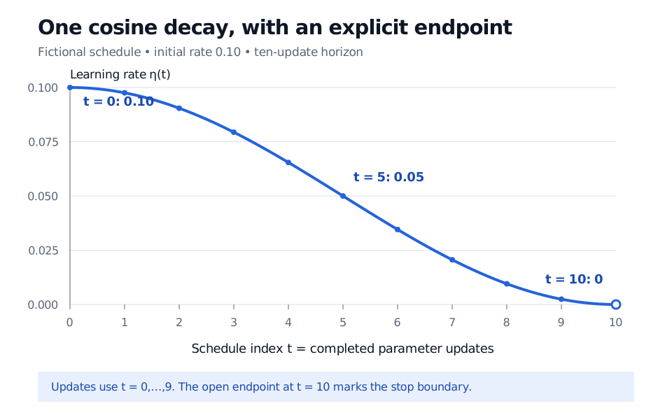
One cosine decay over a ten-update horizon. Filled dots are rates used by updates; the open endpoint is the rate at the stop boundary.
The curve adapts the within-run cosine rule in SGDR, Section 3, equation 5. This example has one decay and no restart. A zero terminal rate is a design choice; other cosine schedules finish at a positive floor.
Warmup, decay and restarts do different jobs
Several choices can be combined, but their names should not be treated as synonyms.
- Step decay holds the rate constant between chosen milestones, then reduces it. The milestones and reduction factors are part of the specification.
- Warmup begins with a smaller rate before reaching the intended training rate. A gradual warmup ramps upward. Goyal and colleagues, Section 2.2, used it to address early optimisation difficulties in large-minibatch ImageNet training; that result is not a guarantee for a financial dataset.
- Warm restarts raise the rate at cycle boundaries and begin another decay. In SGDR the trained parameters are retained, rather than randomly reinitialised. Increasing the learning rate does not erase what the model has learned.
- One-cycle uses an initial rise and fall, followed by a tail below the starting rate in Smith's proposed policy, Section 4.1. It differs from repeatedly restarting a cosine decay.
Batch size also matters. Goyal and colleagues motivate scaling the learning rate in proportion to batch size by assuming gradients change little over the small-batch updates being combined. Their Section 2.1 identifies limits to that approximation. Doubling a batch size is not a universal instruction to double the learning rate.
Compare schedules without spending the test set
Before comparing runs, specify the clock—completed updates, epochs or another explicit measure—along with the initial rate, horizon, warmup, floor and restart boundaries. An epoch is a pass through the training data; changing batch size can change how many updates it contains. Equal epoch counts therefore need not mean equal update counts.
Treat schedule settings as hyperparameters. For a time-ordered financial prediction task, choose them using an earlier training period and an appropriate later validation period, with labels and preprocessing respecting the forecast cutoff. Keep the final test period out of schedule selection. A low training loss or a smooth curve does not establish a global optimum or a useful trading signal.
The SelfMadeQuant lesson Reading Loss Curves connects learning-rate experiments to logged diagnostics and validation-based selection. Its preview is public; the full lesson requires membership.
Sources
- Loshchilov and Hutter (2017), SGDR: Stochastic Gradient Descent with Warm Restarts, introduction and Section 3: gradient updates, step decay, cosine annealing and retained-parameter restarts.
- Goyal and colleagues (2017; revised 2018), Accurate, Large Minibatch SGD: Training ImageNet in 1 Hour, Sections 2.1–2.2: conditional batch-size scaling and gradual warmup.
- Smith (2018), A Disciplined Approach to Neural Network Hyper-Parameters: Part 1, Section 4.1: cyclical rates and the one-cycle policy.