Sparse Gaussian process and inducing points: Definition & Examples

A sparse Gaussian process uses a smaller collection of latent inducing variables to make Gaussian-process inference cheaper. In the inducing-point construction, these variables are function values

u_j=f(z_j)

at locations

Z

. The locations can be selected training inputs or optimized pseudo-inputs; they are not additional observed targets. For a quant fitting a smooth response across many market observations, the benefit is retaining information from the training set through a smaller computational representation. “Sparse” here need not mean a covariance matrix full of zeros. Quiñonero-Candela and Rasmussen, §§2–3.

The small matrix is a bridge

Let $X$ contain $N$ training inputs and $Z$ contain $M$ inducing inputs. Write $K_{XX}$ for the training covariance, $K_{ZZ}$ for the inducing covariance and $K_{XZ}$ for their cross-covariance. Assuming $K_{ZZ}$ is invertible, define

Q_{XX}=K_{XZ}K_{ZZ}^{-1}K_{ZX}.

Its rank is at most

M

. For a zero-mean GP, exact Gaussian conditioning gives

p(f_X\mid u)=\mathcal N\!\left(K_{XZ}K_{ZZ}^{-1}u,\;K_{XX}-Q_{XX}\right).

This identity is not yet an approximation: the residual covariance remains. It describes variation in the training function values that knowing the inducing values does not resolve. GPML, §8.1.

Two inputs, one inducing point

Take unitless training inputs

X=(0,1)

and the RBF kernel with unit variance and length scale,

k(x,x')=\exp\left(-\frac{(x-x')^2}{2}\right).

Place one inducing input at $z=0$ . With $a=e^{-1/2}\approx0.606531$ ,

K_{XX}=\begin{pmatrix}1&a\a&1\end{pmatrix},\qquad K_{XZ}=\begin{pmatrix}1\a\end{pmatrix},\qquad K_{ZZ}=(1),

Q_{XX}=\begin{pmatrix}1&a\a&a^2\end{pmatrix},\qquad K_{XX}-Q_{XX}=\begin{pmatrix}0&0\\0&1-e^{-1}\end{pmatrix}.

The projection has rank one. It reproduces the covariance with $f(0)$ , but represents only $e^{-1}\approx0.367879$ of the unit prior variance at $x=1$ . The remaining $0.632121$ is conditional residual variance. It is neither observation noise nor a fitted forecast-error estimate: no targets have been supplied.

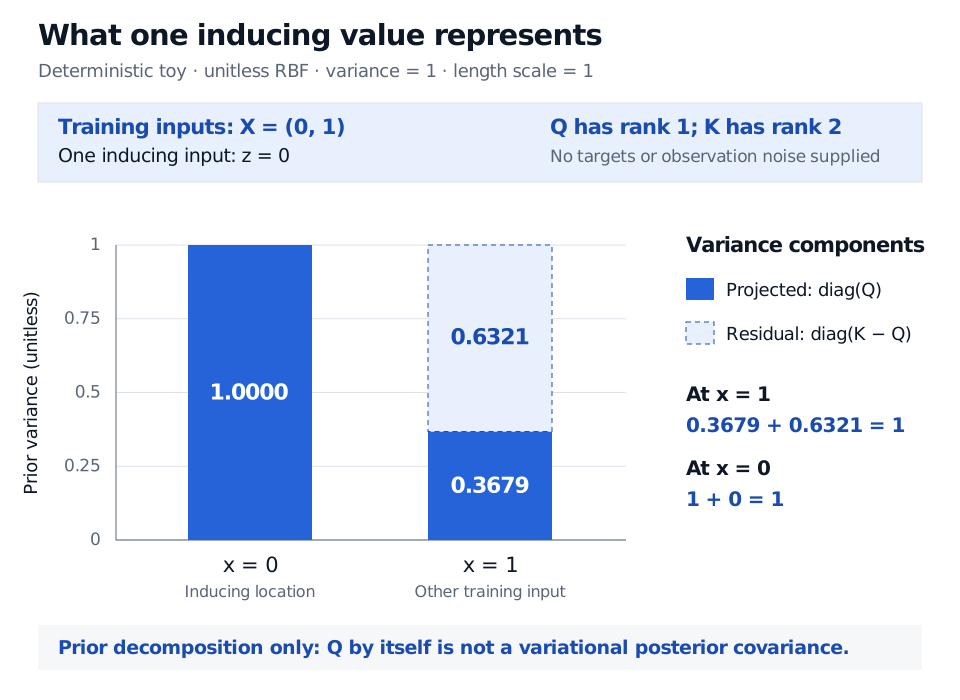
Unitless RBF example with training inputs zero and one and a single inducing input at zero. Each prior variance is one. At zero, the projected component is one and residual variance is zero. At one, the projected component is 0.3679 and residual variance is 0.6321. These are prior components, not posterior uncertainty.

Original deterministic covariance calculation. The inducing value captures one direction of variation; the conditional residual is still part of the GP.

The approximation rule matters

Different sparse methods treat this residual differently. Subset of regressors replaces the covariance by the low-rank projection throughout. DTC retains the exact test conditional but drops training conditional variance; FITC instead retains its diagonal while discarding training conditional correlations. These choices can produce different predictive variances even with identical inducing inputs. See the unifying framework, §§4–6.

In variational inference, one can retain the exact conditional and learn

q(u)=\mathcal N(m,S)

. Defining

A=K_{XZ}K_{ZZ}^{-1}

gives

q(f_X)=\mathcal N\!\left(Am,\;K_{XX}-Q_{XX}+ASA^\top\right).

Thus $Q_{XX}$ alone is not the variational posterior covariance. The posterior also depends on the learned uncertainty about

u

. Keeping

q(u)

explicit permits stochastic training with minibatches when the likelihood factorizes across observations. Hensman et al., §3.1.

For independent Gaussian observation noise with variance $\sigma_n^2>0$ , Titsias's collapsed variational objective is

\mathcal L= \log\mathcal N\!\left(y;0,Q_{XX}+\sigma_n^2I\right) -\frac{1}{2\sigma_n^2}\operatorname{tr}\left(K_{XX}-Q_{XX}\right).

It is a lower bound on the original GP log marginal likelihood. The trace correction penalizes unresolved prior variance relative to observation noise; in our example its numerator is

0.632121

. Optimizing the bound selects inducing locations as variational parameters. Simply replacing

K_{XX}

Q_{XX}

in a Gaussian likelihood omits this correction. Titsias, §3, equations 6–10.

What the speed-up buys

For standard dense algebra and inexpensive kernel evaluations, full-batch inducing-point regression commonly costs

O(NM^2+M^3)

per objective evaluation, versus

O(N^3)

for dense exact regression. Storing the cross-covariance costs

O(NM)

; streaming or minibatch implementations can change memory requirements. These are operation counts, not a bound on total optimization time. Hensman et al., introduction.

After training and suitable precomputation, a common sparse predictive mean costs

O(M)

per test input and its marginal variance

O(M^2)

, excluding kernel-evaluation costs. A full joint covariance over

T

test inputs has

T^2

entries; marginal-variance costs do not describe that larger task. GPML, Table 8.2.

Increasing

M

expands the representation, but selecting a useful number and placement remains an accuracy–cost decision. In financial forecasting, fit inducing locations and hyperparameters within each training window to avoid look-ahead bias. Check predictive coverage on later data: a variational bound does not establish empirical calibration or protect a model from a market regime change.

For the underlying prediction algebra, Gaussian Processes for Regression and Classification provides a public preview; the full lesson requires membership.

Sources

Titsias (2009), Variational Learning of Inducing Variables in Sparse Gaussian Processes, §§2–3: inducing variables, posterior covariance and the trace-corrected bound.
Quiñonero-Candela and Rasmussen (2005), A Unifying View of Sparse Approximate Gaussian Process Regression, §§2–6: distinctions between subset-of-regressors, DTC and FITC approximations.
Hensman, Fusi and Lawrence (2013), Gaussian Processes for Big Data, §§2–3.1: exact conditional, explicit variational inducing distribution and minibatch factorization.
Rasmussen and Williams (2006), Gaussian Processes for Machine Learning, Chapter 8, §§8.1, 8.3 and Table 8.2: precomputation and per-input prediction costs.

The small matrix is a bridge

Two inputs, one inducing point

The approximation rule matters

What the speed-up buys

Sources

Related terms

Look-ahead bias

Matrix rank

Radial basis function kernel

Variational inference and evidence lower bound