Semiparametric model: Definition & Examples

A semiparametric model is a statistical model with both a finite-dimensional parameter component and an infinite-dimensional component, such as an unknown function or distribution. Typically, the finite component describes the effect of interest while the unknown function supplies the rest of the model's structure. “Infinite-dimensional” means that the function is not restricted to a family described by a fixed finite number of coefficients. Sen's notes develop this distinction.

For a credit analyst, this can separate two questions: how a borrower characteristic changes default intensity, and how the underlying intensity varies over the life of the loan. A short vector of coefficients can answer the first while allowing the second to remain flexible.

A coefficient attached to an unspecified curve

The Cox proportional hazards model is a standard example. For a continuous default time $T$ and a fixed borrower characteristic $x$ , write

\lambda(t\mid x)=\lambda_0(t)\exp(\beta x).

Here $\lambda(t\mid x)$ is the hazard rate: the instantaneous default rate conditional on survival to $t$ . If time is measured in years, its units are per year.

Finite component: the coefficient $\beta$ , or a fixed-length coefficient vector with several characteristics.
Function component: the nonnegative baseline hazard $\lambda_0(t)$ , whose time shape is unspecified, subject to the conditions needed for a valid survival law.

The baseline is the hazard for

x=0

throughout time; it is not just the hazard at time zero. Choosing a constant baseline would produce a parametric submodel. Leaving the baseline function unspecified gives the semiparametric formulation. The model still imposes structure: with fixed covariates, their hazard multiplier is constant over time. These are the ingredients described in ISL §§11.5.1–11.5.2.

Twice the hazard, 3.96% default risk

Consider a synthetic physical default model with binary

x

x=0

identifies a reference borrower group and

x=1

another group. Default is the only event ending survival in this example. Stipulate

\beta=\log 2

. Wherever the baseline hazard is positive,

\frac{\lambda(t\mid 1)}{\lambda(t\mid 0)}=\exp(\beta)=2.

This is a ratio of instantaneous rates among the borrowers still surviving at time $t$ . To get a probability over an entire year, we also need baseline survival information.

Let

H_0(t)=\int_0^t\lambda_0(s)\,ds

be the cumulative hazard and

S_0(t)=\exp[-H_0(t)]

the baseline survival function. Integrating the scaled hazard gives

S(t\mid x)=\exp[-\exp(\beta x)H_0(t)] =S_0(t)^{\exp(\beta x)}.

Now supply one additional anchor: $S_0(1\text{ year})=0.98$ . Then

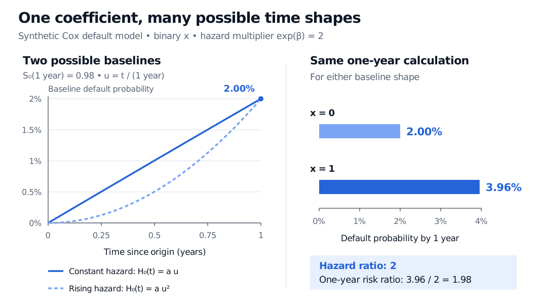
\begin{aligned} S(1\text{ year}\mid 1)&=0.98^2=0.9604,\\ \mathbb{P}(T\le 1\text{ year}\mid x=0)&=1-0.98=0.02,\\ \mathbb{P}(T\le 1\text{ year}\mid x=1)&=1-0.9604=0.0396. \end{aligned}

The one-year default risks are 2% and 3.96%. Their risk ratio is

0.0396/0.02=1.98

, and the increase is 1.96 percentage points. A hazard ratio of two does not exactly double the one-year probability. In this particular case, the identity

1-S_0^2=(1-S_0)(1+S_0)

explains the risk ratio

1+0.98=1.98

Two baseline default curves sharing a 2 percent one-year endpoint, alongside one-year group default probabilities of 2 percent and 3.96 percent.

Original synthetic illustration. Two selected baseline shapes share the same one-year survival anchor; neither shape is imposed by the semiparametric Cox model. Both give the same one-year group risks.

For the picture, let $u=t/(1\text{ year})$ and $a=-\log(0.98)$ . The illustrative cumulative hazards $H_0(t)=au$ and $H_0(t)=au^2$ agree at one year while producing different default probabilities before it. Their derivatives are nonnegative; the rising-hazard illustration starts with zero instantaneous hazard. The multiplicative model remains valid there, although a ratio of its two zero hazards is undefined. One survival anchor fixes the cumulative hazard at that horizon, without specifying the whole baseline function.

What flexibility buys—and what remains to check

Cox's partial likelihood uses the relative hazards within each event-time risk set. The shared baseline cancels, allowing estimation of

\beta

without choosing a parametric baseline shape, under the model and suitable observation assumptions, including conditionally independent censoring. Censored borrowers contribute while they remain at risk. Correct handling of censoring, tied event times and the risk sets still matters; the R coxph documentation describes the fitting machinery.

Absolute default predictions require baseline survival information as well as coefficients. After fitting, that information can be estimated from the data; the baseline need not be assigned a parametric form to obtain survival curves. See the official survfit.coxph documentation.

An unspecified baseline does not remove the proportional-hazards restriction or protect a misspecified covariate effect. Time-varying effects require investigation and possibly a different specification; cox.zph provides diagnostics. A fitted association also does not establish that changing

x

causes default risk to change: confounding and selection remain substantive concerns.

For the hazard-to-survival derivation and the distinction between physical default forecasts and risk-neutral pricing probabilities, continue with Reduced-Form Models: Hazard Rates and Risk-Neutral Default Probabilities (membership lesson; public preview). The synthetic probabilities above have a physical forecasting interpretation; a pricing calculation requires an appropriate risk-neutral model.

Sources

Bodhisattva Sen, Semiparametric Statistics, Columbia University notes, 4 April 2018, introduction and Example 4.2.
Gareth James, Daniela Witten, Trevor Hastie and Robert Tibshirani, An Introduction to Statistical Learning with Applications in R, second edition, 2021, §§11.5.1–11.5.2 and 11.7.4.
R survival documentation: coxph, survfit.coxph and cox.zph.

A coefficient attached to an unspecified curve

Twice the hazard, 3.96% default risk

What flexibility buys—and what remains to check

Sources

Related terms

Parametric model

Statistical model

Survival function