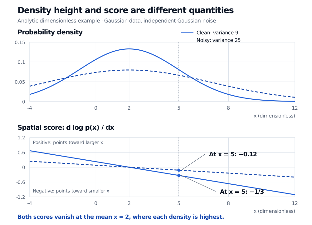
Score-based generative model: Definition & Examples

A score-based generative model learns the gradient of a data distribution's log density and uses that learned field in a sampling procedure. For a quant building synthetic market scenarios, the object being learned is a direction in the space of possible observations, rather than a predicted return or an event probability. Song and Ermon, §2.

What the score measures

For a smooth, positive density $p(x)$ , the spatial score is

s(x)=\nabla_x\log p(x).

It points toward the steepest local increase in log density. In several dimensions it has one component per data coordinate. The derivative is with respect to the observation $x$ ; it differs from the parameter score

\nabla_\theta\log p_\theta(x)

used in likelihood estimation.

Neither

p(x)

nor

\log p(x)

is the score. A score can be negative, and zero score does not imply zero density. If

p(x)=q(x)/Z

, where

Z

is constant in

x

, then

\nabla_x\log p=\nabla_x\log q

: the normalising constant drops out. This is why a score can be learned without first evaluating a normalised density. Yang Song's author tutorial, “The score function”.

Consider a fictional dimensionless feature with Normal distribution,

X\sim\mathcal{N}(2,9)

. Here 9 is the variance, so the standard deviation is 3. Differentiating its log density gives

\log p(x)=-\tfrac12\log(18\pi)-\frac{(x-2)^2}{18}, \qquad s(x)=-\frac{x-2}{9}.

At $x=5$ , the score is $-1/3$ : a small movement toward smaller $x$ raises the density. At the mean $x=2$ , the score is zero even though the density is at its maximum.

Now add independent noise $\epsilon\sim\mathcal{N}(0,16)$ . The noisy feature $Y=X+\epsilon$ has variance $9+16=25$ and score

s_Y(y)=-\frac{y-2}{25},\qquad s_Y(5)=-\frac{3}{25}=-0.12.

This is the score of the noisy marginal distribution. It is not the clean score evaluated on a noisier observation. At the same coordinate 5, smoothing has changed the field itself.

Analytic dimensionless Normal example: clean mean 2 and variance 9 versus noisy mean 2 and variance 25. Both densities peak at 2 and both scores are zero there. At x equals 5, the clean score is minus one third and the noisy score is minus 0.12.

Original analytic example. The upper panel shows density height; the lower panel shows its log derivative. Independent noise of standard deviation 4 broadens the density and flattens the score field.

A trainable target without the unknown density

Score matching fits a network

s_\theta

to the data score. The unknown true score prevents directly evaluating the ideal squared-error loss. Denoising score matching supplies a computable target by corrupting training observations.

For Gaussian corruption $\tilde x=x+\sigma z$ , with $z\sim\mathcal{N}(0,I)$ and $\sigma>0$ , the conditional corruption score is

\nabla_{\tilde x}\log p(\tilde x\mid x) =-\frac{\tilde x-x}{\sigma^2}=-\frac{z}{\sigma}.

One trains across noise levels using a positively weighted loss such as

\mathbb{E}_{\sigma,x,z}\left[ \lambda(\sigma)\left\lVert s_\theta(x+\sigma z,\sigma)+\frac{z}{\sigma} \right\rVert^2\right].

Although each target uses a known corruption draw, the population optimum estimates the marginal noisy-data score, not the score of one observation's corruption kernel. Conditioning on noise level lets one network learn a family of fields. Added noise also smooths distributions concentrated on lower-dimensional structures. These are population statements with regularity and capacity assumptions; finite training gives an approximation. Song and Ermon, §§2.1 and 3–4.

Generation needs a sampler and a clock

Following a score uphill alone does not sample its density. In the clean Normal example, repeatedly applying the deterministic update $x\leftarrow x+s(x)$ moves points toward 2. Even starting with the correct distribution, one step reduces its variance from 9 to $64/9\approx7.1111$ ; repeated steps collapse it toward the mode.

A basic Langevin discretisation instead combines drift and randomness:

x_{k+1}=x_k+h\,s_\theta(x_k)+\sqrt{2h}\,z_k, \qquad z_k\sim\mathcal{N}(0,I).

For an exact score, the corresponding continuous-time Langevin process has the target density as its invariant distribution under suitable conditions. Finite steps and finite running time introduce discretisation and convergence errors. Annealed Langevin sampling changes from large-noise fields to smaller-noise fields; it is not merely optimisation of the clean density. Song's tutorial, “Langevin dynamics” and “Multiple noise perturbations”.

The continuous diffusion formulation starts from the forward stochastic differential equation

dX_t=f(X_t,t)\,dt+g(t)\,dW_t,

where

g(t)

is a scalar, spatially constant diffusion coefficient. Write

p_t

for the marginal density. With the original clock running backwards, the reverse equation is

dX_t=\left[f(X_t,t)-g(t)^2\nabla_x\log p_t(X_t)\right]dt +g(t)\,d\bar W_t,\qquad t:T\to0.

Here $dt<0$ ; the reverse Brownian increment has covariance $|dt|I$ . Equivalently, with an increasing reverse clock $\tau=T-t$ and $Y_\tau=X_{T-\tau}$ , the drift becomes

dY_\tau=\left[-f(Y_\tau,T-\tau) +g(T-\tau)^2\nabla_y\log p_{T-\tau}(Y_\tau)\right]d\tau +g(T-\tau)\,dB_\tau.

The signs differ because the clock differs. Substituting a learned score and starting from a tractable approximation to

p_T

gives a numerical generator; score error, terminal-distribution mismatch and solver error affect its output. These formulas do not cover state-dependent diffusion coefficients without additional terms. Song et al., §§3.1–3.3 and 4.1.

For market data, diffusion time indexes artificial corruption, not elapsed trading time. A whole return window can be one observation. Generated paths still need chronological holdout checks for tails, cross-asset dependence and conditioning information available at the scenario date. Learning a score imposes no arbitrage restriction by itself. See diffusion models for financial data for the application boundary and DDIM for a different sampling construction.

Sources

Song and Ermon (2019), Generative Modeling by Estimating Gradients of the Data Distribution, §§2–4: score estimation, denoising score matching, noise conditioning and annealed Langevin sampling.
Song et al. (ICLR 2021), Score-Based Generative Modeling through Stochastic Differential Equations, §§3.1–3.3 and 4.1: forward and reverse SDEs, the negative-time-step convention, training and numerical solution. Version read dated 10 February 2021.
Yang Song (2021), Generative Modeling by Estimating Gradients of the Data Distribution, author tutorial: spatial scores, normalisation, Langevin dynamics and multiple noise scales.

What the score measures

A trainable target without the unknown density

Generation needs a sampler and a clock

Sources

Related terms

Denoising diffusion implicit model

Normal distribution

Stochastic differential equation