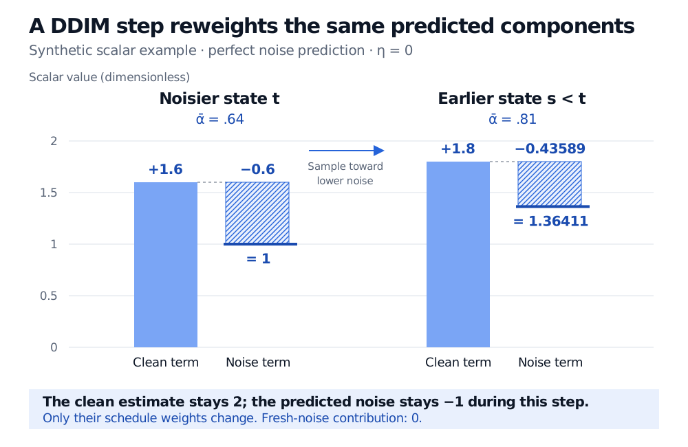
DDIM reuses a diffusion noise predictor to sample along a chosen time grid. With eta zero, updates are deterministic given the initial noise, but generated samples remain random.
Denoising diffusion implicit model
A denoising diffusion implicit model (DDIM) generates data by repeatedly applying a trained diffusion noise predictor, with a sampling rule that can omit intermediate noise levels. Its usual deterministic form adds no fresh noise during these updates. For a quant experimenting with synthetic market scenarios, this offers a way to reduce generation cost; it does not establish that the resulting scenarios have realistic financial tails or dependence. Song, Meng and Ermon, §§4.1–4.2.
Read the clock before the update
Diffusion time indexes noise level, not trading time. A whole return window could be one observation x0; the index t then describes how much artificial noise has been added to that window.
In the usual DDPM notation, let βt be the forward noise variance, αt=1−βt, and
αˉt=j=1∏tαj,αˉ0=1.
The bar matters: αˉt is cumulative signal retention, not one step's retention. The forward marginal can be sampled as
xt=αˉtx0+1−αˉtϵ,ϵ∼N(0,I).
Here I is the identity covariance; for a scalar it is 1. Increasing t reduces αˉt and increases the noise weight. Generation runs the other way: from a noisy state t to an earlier state s<t, where αˉs>αˉt. These conventions follow Ho, Jain and Abbeel, §2; the DDIM paper writes the cumulative quantity as αt without a bar.
A network ϵθ(xt,t) learns to predict the injected noise across noise levels using a squared-error objective. The standard-normal draw used to corrupt a training observation is known during training; it must be inferred at generation time. Ho et al., §3.4.
Estimate clean data, then move to less noise
Write ϵ^=ϵθ(xt,t). The predicted clean observation is
x^0=αˉtxt−1−αˉtϵ^.
For a chosen earlier sampling time s, the generalised update is
Take 0≤η≤1 here. At η=0, the final random term disappears, leaving a weighted clean estimate and a retained predicted-noise direction. The noise-direction term generally remains nonzero. At η=1, this variance choice gives a DDPM-type stochastic update on the selected grid; it does not describe every DDPM variance convention. The authors' reference implementation computes these three components explicitly.
For a fixed predictor, conditioning inputs and grid, zero-noise updates are deterministic given the starting state. Sampling normally begins with random xT∼N(0,I), so repeated draws of that initial state still generate a distribution of outputs.
One scalar step you can audit
Use an artificial dimensionless clean value x0=2 and stipulated noise ϵ=−1. With αˉt=0.64,
xt=0.8(2)+0.6(−1)=1.
Assume a perfect predictor returns ϵ^=−1. It recovers
x^0=0.81−0.6(−1)=2.
Now choose an earlier noise level with αˉs=0.81. The deterministic update is
xs=0.9(2)+0.19(−1)=1.3641101056…
The scalar has increased while becoming less noisy: denoising need not decrease a coordinate's value. This calculation stipulates the correct noise; a real trained predictor does not receive the original clean value or its corruption draw. Exact recovery here is an assumption of the toy, not a DDIM guarantee.
Synthetic perfect-predictor DDIM step with eta zero: at alpha-bar 0.64, clean contribution 1.6 plus noise contribution minus 0.6 gives 1. At alpha-bar 0.81, 1.8 minus 0.43589 gives 1.36411. Fresh-noise contribution is zero.
Original dimensionless scalar example, not a fitted financial model. The predicted clean value and noise are held fixed for one update; their schedule weights change.
What fewer steps change
DDIM changes the sampling construction while reusing the DDPM denoising objective. Its derivation uses alternative, non-Markovian forward joint distributions with the same noisy-data marginals. This does not mean the generated update needs the entire past trajectory: the displayed rule uses the current state and predictor.
A shorter selected time grid requires fewer sequential network evaluations. With an imperfect predictor, changing the grid can change the final output even for identical initial noise. The original image experiments demonstrate a speed–quality trade-off, not universal accuracy at any step count. DDIM, §§3–5.
For a financial diffusion generator, evaluate the chosen sampling grid on held-out periods, including joint dependence, tail events and downstream risk calculations. Keep conditioning information and preprocessing within the relevant historical cutoff. Faster sampling cannot correct a misspecified training distribution or information leakage. Nor does the denoising clock itself define an arbitrage-free price process.
Sources
Song, Meng and Ermon, Denoising Diffusion Implicit Models, §§3–5: shared denoising objective, deterministic sampling, selected trajectories and experimental limitations. First posted 2020; ICLR 2021; version read dated 5 October 2022.