Skip to content

Root mean squared error

RMSE puts squared forecast errors back in the target’s units. See why equal mean absolute errors can give different RMSEs, and which denominator to use.

Root mean squared error (RMSE) is the square root of the average squared error. For nn observed values yiy_i and their predictions y^i\hat y_i, the usual empirical score is
RMSE⁡=1n∑i=1n(yi−y^i)2=MSE⁡.\operatorname{RMSE} =\sqrt{\frac1n\sum_{i=1}^{n}(y_i-\hat y_i)^2} =\sqrt{\operatorname{MSE}}.
Taking the root restores the target's units: when slippage errors are in basis points, mean squared error is in basis points squared and RMSE is in basis points. A trading desk can therefore report forecast accuracy on the same scale as its execution costs, while retaining squared error's strong penalty for large misses.
The order of operations matters: square each error, average the squares, then take one square root. Taking each square root before averaging gives the mean absolute error (MAE), because ei2=∣ei∣\sqrt{e_i^2}=\lvert e_i\rvert. That is a different score.

A zero average error can still hide large misses

Suppose two models forecast slippage for the same four synthetic orders. Define the signed error as realised slippage minus forecast slippage; a negative error means the forecast overstated the realised cost.

OrderModel A error (bps)A squared error (bps²)Model B error (bps)B squared error (bps²)
1−2-244−1-111
21111−1-111
311111111
400001111

Both models have mean signed error zero and MAE of 11 basis point. Their RMSEs differ:

RMSE⁡A=4+1+1+04=32≈1.225 bps,RMSE⁡B=1+1+1+14=1 bps.\operatorname{RMSE}_A=\sqrt{\frac{4+1+1+0}{4}} =\sqrt{\frac32}\approx1.225\text{ bps}, \qquad \operatorname{RMSE}_B=\sqrt{\frac{1+1+1+1}{4}}=1\text{ bps}.

Model A's single −2-2 basis point miss contributes 44 of its 66 basis points squared of total error. Model B spreads its absolute error evenly. RMSE prefers B on these observations, even though MAE ties. Neither score tells us whether underestimating costs is more damaging than overestimating them: squaring erases the sign.
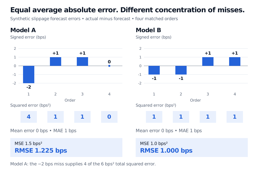
Synthetic four-order errors in basis points. Model A has errors minus 2, 1, 1, 0; Model B has minus 1, minus 1, 1, 1. Both have zero mean error and MAE 1 bps. Model A has MSE 1.5 bps squared and RMSE 1.225 bps; B has MSE 1 and RMSE 1 bps.
Original synthetic comparison, not market data. The signed bars show cancellation; the squared-error ledger shows why concentrating the same total absolute error in a larger miss raises RMSE.

For the same unweighted observations, RMSE is at least MAE; equality holds when all absolute errors are equal. It is also nonnegative and is zero exactly when every scored error is zero. It is not the average error magnitude in the ordinary arithmetic sense, nor is it the largest error or a bound on the next error.

What the root changes—and what it preserves

On the same evaluation cases, minimising RMSE gives the same ranking as minimising MSE: square root is strictly increasing. The root changes the reporting scale, not which prediction vector wins. A return forecast expressed in decimal returns will have a numerically different RMSE from the same forecast expressed in basis points; model comparisons need consistent units, targets and horizons.

A population version is

RMSE⁡=E[E2],\operatorname{RMSE}=\sqrt{\mathbb{E}[E^2]},

where EE is a random prediction error with a finite second moment. It differs from E[∣E∣]\mathbb{E}[\lvert E\rvert]. Its squared value satisfies

E[E2]=Var(E)+(E[E])2.\mathbb{E}[E^2]=\text{Var}(E)+(\mathbb{E}[E])^2.
Thus a persistently biased forecast and a variable forecast can both have a large RMSE. With zero mean error, population RMSE equals the error's standard deviation. Empirically, the analogous identity uses error variance with divisor nn, not the usual n−1n-1 sample-variance convention. In the example, a mean error of zero removes systematic offset on those four orders; it does not remove their dispersion or establish unbiased future forecasts.

Count scored cases, or estimate a noise variance?

The nn in empirical RMSE is the number of scored cases. It does not become n−1n-1 just because predictions came from a fitted model.

A different question arises when estimating the disturbance variance in an ordinary linear regression. With pp fitted coefficients including the intercept, a full-rank design, n>pn>p, a correctly specified conditional mean and conditionally uncorrelated disturbances of common variance σ2\sigma^2, the familiar estimator is

s2=RSS⁡n−p,RSS⁡=∑i=1nei2.s^2=\frac{\operatorname{RSS}}{n-p}, \qquad \operatorname{RSS}=\sum_{i=1}^{n}e_i^2.

This degrees-of-freedom correction makes s2s^2 unbiased for σ2\sigma^2 under those assumptions. The residual standard error is s=RSS⁡/(n−p)s=\sqrt{\operatorname{RSS}/(n-p)}; taking its root does not itself make ss an unbiased estimator of σ\sigma. Empirical training RMSE remains RSS⁡/n\sqrt{\operatorname{RSS}/n}. For simple regression with an intercept, p=2p=2.

Always read the stated convention: some regression reports use “root MSE” for the degrees-of-freedom-adjusted residual standard error. A number and a label alone may not identify which denominator was used.

A useful forecast report needs more than one number

Evaluate competing models on the same later observations, using only information available at each forecast origin. A low training RMSE can reflect overfitting; the same formula on genuinely held-out observations answers a more useful forecasting question. A few large misses can dominate the score, so retain the signed errors and consider whether an asymmetric or tail-sensitive loss function better matches the decision.
Forecast Evaluation develops rolling and expanding evaluation designs and comparisons under squared or absolute error. The linked page is a public preview; the full lesson requires membership. Lower RMSE on a chosen test set remains a statistical comparison, not a guarantee of stable trading value after costs.

Sources

  • Christopher M. Bishop, Pattern Recognition and Machine Learning, Springer, 2006, §1.1, pp. 6–8, especially equation (1.3): RMS error, original target units and separate training/test evaluation.
  • Gareth James, Daniela Witten, Trevor Hastie, Robert Tibshirani and Jonathan Taylor, An Introduction to Statistical Learning: with Applications in Python, Springer, 2023, §3.1.2, pp. 75–76: disturbance assumptions and residual standard error with denominator n−2n-2 in simple linear regression.
  • Rob J Hyndman and George Athanasopoulos, Forecasting: Principles and Practice, third edition, §5.8: test-set errors, scale-dependent metrics and the RMSE/MAE distinction.
  • scikit-learn documentation, root_mean_squared_error: regression scoring API, nonnegative score and zero-error optimum.
Last updated
  • forecasting
  • prediction
  • error metrics
  • model evaluation
← Back to the glossaryBack to top ↑