How random assignment supports a causal comparison, why intention-to-treat matters, and why an unbiased experiment can still give a misleading realised difference.
Randomised controlled experiment (A/B test)
A randomised controlled experiment assigns units to a treatment and a comparison condition using a known chance mechanism, then compares their outcomes. An A/B test is the two-condition version. For a quant team, random assignment can distinguish the effect of a platform change from the tendency of particular users or orders to receive it. A control group selected by user choice does not supply the same protection against confounding. J-PAL’s randomisation guide explains the design’s conceptual basis.
What is being randomised?
Specify the eligible units, the two interventions, the outcome and its measurement window before assigning anyone. Record the assignment probabilities. Complete randomisation fixes the number in each arm and chooses that many units uniformly; flipping a coin independently for each unit generally leaves the arm sizes random. Known unequal probabilities or blocking require analysis appropriate to that design. J-PAL distinguishes the lottery and fixed-count procedures.
The assignment unit receives the random draw; the analysis unit is the record being analysed. A desk assigned one execution rule might generate thousands of trade records. Those rows do not become thousands of separately randomised desks. Athey and Imbens, §8 explain why the design and the desired weighting matter in clustered experiments.
A completion-rate experiment
Consider a fictional finance-research platform with 100 participants, one observation per participant, no interaction between them and complete follow-up. It randomly assigns exactly 50 to a new onboarding prompt and 50 to the current prompt. Success means completing the same specified research task within seven days. This is a platform outcome, not a trading-return claim.
Original assignment
Completed
Did not complete
Completion rate
A: new prompt
30
20
60%
B: current prompt
20
30
40%
Keeping participants in their original groups gives an intention-to-treat comparison: the effect of assignment to the prompt, including any failure to use it. Moving non-users into the control arm instead conditions on behaviour after assignment. Randomisation does not justify that comparison. Athey and Imbens, §9.1 define this assignment effect.
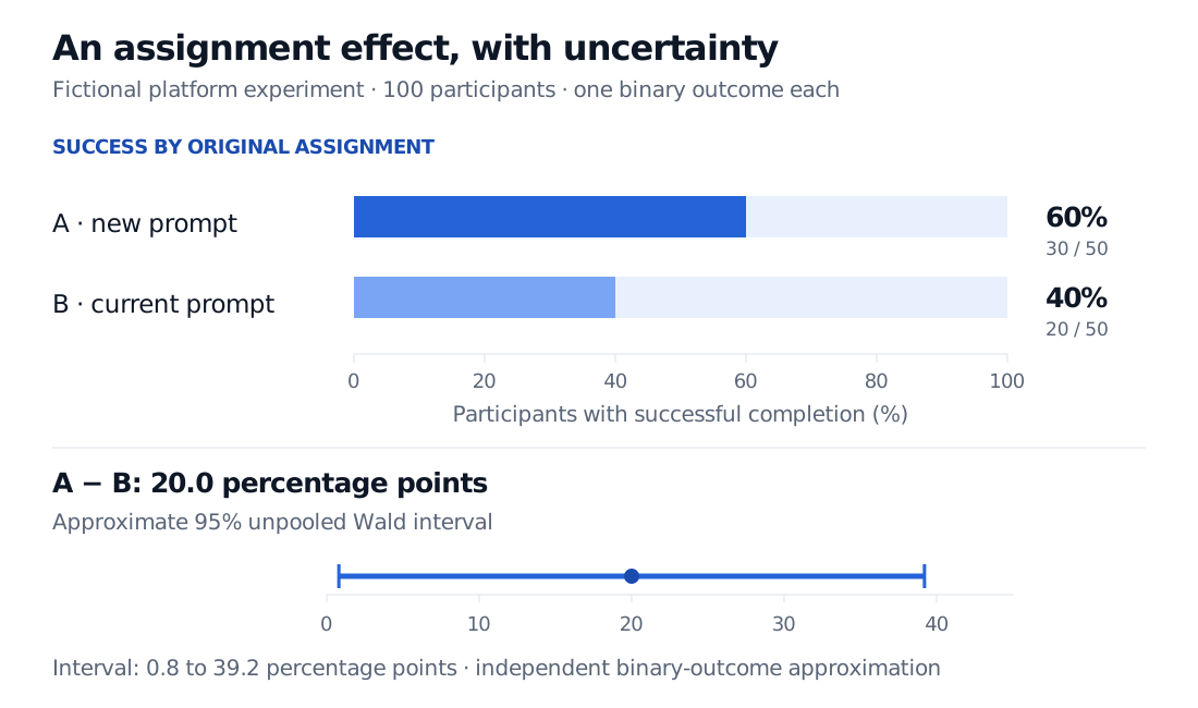
The estimated difference is 0.60−0.40=0.20, or 20 percentage points. The ratio is 0.60/0.40=1.5: a 50% relative increase in completion, not a 50-percentage-point increase. The binary-outcome term risk difference also refers to this difference in event probabilities; here the event is successful completion.
For an illustrative calculation, model the outcomes as independent Bernoulli observations within and across arms, with a common success probability within each arm. The unpooled standard error is
SE=500.60(0.40)+500.40(0.60)=0.0096≈0.09798.
The normal-approximation 95% confidence interval, using z0.975≈1.959964, is
0.20±z0.975(0.09798)≈[0.00796,0.39204].
That is roughly 0.8 to 39.2 percentage points, a wide interval. NIST's Wald formula gives this calculation and warns that its coverage can fall below the nominal level. It is not an exact randomisation interval. In the finite-population framework below, assignments are dependent when arm sizes are fixed; random assignment alone does not establish this independent-outcome model. Design-based variance estimation is a separate calculation.
Fictional experiment: 30 of 50 participants assigned the new prompt complete the task, versus 20 of 50 controls. The estimated difference is 20 percentage points, with an approximate 95% unpooled Wald interval from 0.8 to 39.2 percentage points.The two rates use original assignments. The interval adds an independent binary-outcome approximation to the experimental design.
Why unbiased does not mean exactly right
Let Yi(1) and Yi(0) be participant i's potential outcomes under the two assignments. Only one is observed. The finite-sample average treatment effect is
τN=N1i=1∑N(Yi(1)−Yi(0)).
With fixed potential outcomes, complete randomisation and positive arm sizes, the difference of observed means τ^ obeys EZ[τ^]=τN. The expectation is over the assignment mechanism, not a claim that this run reveals the missing outcomes. Miratrix, Sekhon and Yu, §2 develop this finite-population framework.
The model needs well-defined treatment versions and no interference between units, often grouped under SUTVA, the stable unit treatment value assumption. Otherwise Yi(z) alone may not specify the outcome. Recht's potential-outcomes notes, §§1–3 explain the no-interference restriction and assignment-based unbiased estimation.
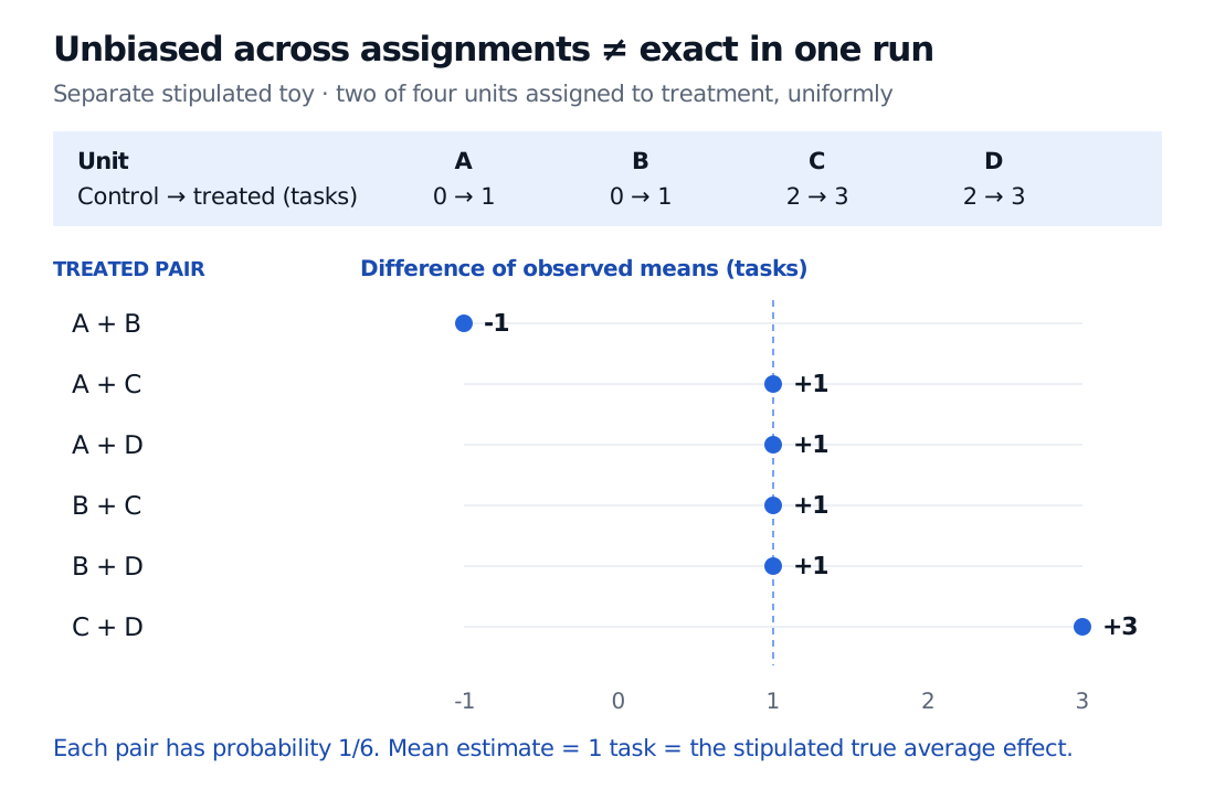
A separate, fully stipulated toy makes the distinction visible. Four units A–D would complete respectively 0, 0, 2 and 2 tasks under control, and 1, 1, 3 and 3 under treatment. Every individual effect is exactly one task. Choose two treated units uniformly from the six possible pairs. The six observed differences are −1,1,1,1,1,3; their average is one. The A+B assignment produces an estimate of minus one even though treatment helps every unit.
Six equally likely treated pairs in a stipulated four-unit experiment produce observed mean differences of minus one, one, one, one, one and three tasks. Their mean is one task, equal to the stipulated true average effect.Every pair has probability one sixth. Unbiasedness averages over all six assignments; it does not promise covariate balance or the correct sign in every realised experiment.
Where implementation changes the interpretation
An execution experiment can have interference and spillovers: one order changes liquidity faced by another. Assigning groups or time blocks may help, but requires its own design and assumptions. More observations within one assignment group do not repair a lack of independent assignment units.
Keep outcome measurement comparable, use blinding where feasible, and specify how missing outcomes, repeated metric inspection and the stopping rule will be handled. J-PAL’s pre-analysis guidance explains how recording analysis choices limits specification searching. An intention-to-treat label does not recover outcomes lost through selective attrition. Random assignment also does not make volunteer users representative of every future user or market regime. These implementation and generalisation limits are separate from the random draw itself. Athey and Imbens, §§2.2–2.4, 4.3 and 8–9 discuss the corresponding distinctions.
The experiment is the data-generating design. A randomisation test is an inferential procedure using assignments allowed by that design under a specified null. Neither is interchangeable with simply shuffling arbitrary rows.
For a comparison design without random assignment, the Difference-in-Differences lesson explains the additional parallel-trends argument and the distinction between treatment categories and assignment clusters. A public preview is available; the full lesson requires membership.
Practice: count the random draws
Twelve desks are randomised, five to a new protocol and seven to the current one. Each desk contributes 40 trade records. Does analysing 480 rows create 480 separately randomised units?
Answer. No. There are 12 assignment units and 480 trade-level analysis records: 200 from treated desks and 280 from controls. A trade-level analysis must respect desk-level assignment and the relevant dependence. Twelve desks also need not provide enough information for a reliable large-cluster approximation. Counting rows cannot establish that approximation.