Policy learning chooses actions to maximise causal value within feasible rules. See how costs, capacity and independent evaluation change treatment decisions.
Policy learning and optimal treatment rules
Policy learning uses data to choose a rule that assigns actions to maximise expected causal benefit within operational constraints. An optimal treatment rule is the best rule for the stated objective and feasible set. For a quant allocating a limited customer-service intervention, predicting which customers will generate the most revenue is a different task from deciding whose revenue the intervention would improve.
From an effect to a decision
Let X denote information available before assignment, and let Y(1) and Y(0) be outcomes with and without an action. A binary rule π(X) chooses whether to act. Write the conditional average treatment effect as τ(x)=E[Y(1)−Y(0)∣X=x]. If Y excludes an incremental action cost c(x), the expected gain relative to taking no action is
G(π)=E[π(X){τ(X)−c(X)}].
Costs and outcomes must share units and a horizon; costs already included in Y must not be subtracted twice. Without constraints, and with known effects, act where τ(x)>c(x), with ties indifferent. With restrictions, solve
π∗∈argmaxπ∈ΠG(π),
where Π contains permitted rules. Budget, simplicity and allowed-feature restrictions can change this set. Regret is the value shortfall G(π∗)−G(π^) relative to its best rule. “Optimal” therefore depends on what is feasible. Athey and Wager, §§1–2 develop this constrained policy-value perspective.
Two positive opportunities, one available place
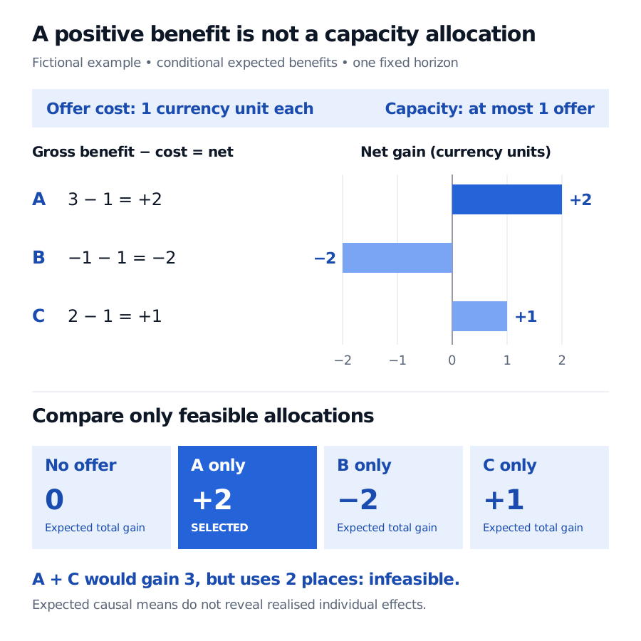
Consider a fictional batch of three customers eligible for a service offer. The objective is total expected incremental profit over one fixed horizon. Conditional gross benefits are stipulated as causally identified and known; each offer costs one currency unit. At most one customer can receive an offer.
Customer
Conditional gross benefit
Offer cost
Conditional net benefit
A
3
1
+2
B
−1
1
−2
C
2
1
+1
The feasible allocations are no offer, A only, B only, or C only. Their total expected gains are respectively 0, 2, −2 and 1. Choose A only. Acting on every positive net benefit would choose A and C and violate capacity. Treating everyone would produce total expected net gain 1 but would also be infeasible.
Fictional three-customer allocation. Gross conditional benefits 3, minus 1, and 2 less cost 1 give net benefits plus 2, minus 2, and plus 1 currency units. With at most one offer, select customer A for total expected gain 2; selecting A and C would exceed capacity.
Original fictional allocation with stipulated causal conditional means. The feasible optimum selects A; positive net benefit alone does not make C feasible alongside A. Values are expected gains, not realised individual effects.
These are conditional averages assigned to customer features, not three observable individual causal gains. This batch illustrates allocation after effects are supplied; it does not demonstrate successful learning. A repeated allocation rule must take competing candidates and remaining capacity into account. A limit on the expected treatment rate alone does not enforce a hard limit in every batch. With unequal resource requirements, simply sorting by net benefit need not solve the constrained problem.
The evidence must identify an intervention
The binary model needs well-defined actions and consistency. In observational data, conditional exchangeability must justify comparison after adjusting for pre-action features, and positivity requires support for the actions being compared. The simple value expression also excludes unmodelled spillovers. These conditions underlie the selection-on-observables setup in Athey and Wager, §2.1.
For example, an unrecorded warning may cause both a service offer and subsequent customer departure. Good departure prediction would not establish the offer's effect. If one offer displaces another customer's service or changes market prices, an isolated-customer effect may also fail to represent deployment value.
Learn the rule, then assess its value
An effect model followed by a threshold is one approach. Another optimises a policy objective directly using estimated causal reward scores within a restricted class, such as shallow trees. The official policytree examples demonstrate doubly robust scores, tree-based action assignment and predictions on held-out observations. A compact rule can sacrifice flexibility to make decisions implementable.
Evaluation asks what the chosen rule would earn under its own assignments. Historical records reveal only the outcome of the action actually taken. Off-policy evaluation must account for the difference between historical assignments and the proposed rule. Doubly robust evaluation combines an outcome model with a correction based on assignment probabilities; its bias protection requires suitable correctness of the outcome or assignment model, alongside identification and support. Small assignment probabilities can still make evaluation noisy. Dudík, Langford and Li, §§2–4 derive these properties.
Use cross-fitting to separate nuisance estimation from score construction, and preserve independent data for assessing the selected rule. Cross-fitting alone does not turn the largest value found during policy search into an unbiased final performance estimate. Report uncertainty, the comparison rule and capacity use; close estimated gains may not support a reliable ranking. The official policytree vignette, Example 3 explicitly separates policy fitting and held-out evaluation.
For financial histories, Time-Ordered Train, Validation and Test Design (membership; public preview) explains how fitting, selection and final confirmation must respect outcome availability. Even a sound historical causal estimate may cease to describe a changed customer mix or intervention. The one-step rule here also does not optimise a sequence of actions that changes future states, the setting addressed by reinforcement learning.