The Phillips curve describes how wage or price inflation tends to respond to pressure on the economy’s productive capacity. In a price Phillips curve, firms facing stronger demand and tighter capacity tend to raise prices faster, holding expected inflation and supply conditions fixed. A macro analyst can use the relationship to test whether an inflation scenario fits the assumed path for demand, costs and expectations. Furlanetto and Lepetit (2024), Sections 1–2
A. W. Phillips studied nominal wage growth and the unemployment rate in the United Kingdom from 1861 to 1957. He found that wages generally rose faster when unemployment was low. Modern price formulations explain the rate of change of a price index and typically allow for inflation expectations and cost pressures. Wage growth and price inflation can diverge when productivity or other input costs change. Phillips (1958), Sections I, II and V, Furlanetto and Lepetit (2024), Sections 1–2
One year, three contributions
Let be price inflation over year , measured as a percentage change in the price index from the end of year to the end of year . In this simplified expectations-augmented model, is the inflation expectation for that same index and year, formed at the end of the preceding year.
The output gap is the same year’s real GDP minus potential output, divided by potential output and expressed in percent. A positive gap means production is above estimated sustainable capacity. With , each percentage point of additional gap adds percentage points (pp) to inflation. The term is the year’s net cost-push contribution in pp. An unexpected rise in imported input costs can make it positive. This is a conditional scenario equation. To use it before year-end, the analyst needs assumptions or forecasts for the year’s gap and cost shock. Furlanetto and Lepetit (2024), Sections 1–3
The sign reverses if the horizontal axis is the unemployment gap, defined as actual unemployment minus its estimated benchmark. A positive unemployment gap indicates spare labour capacity. The gap version of Okun's Law explains why above-potential output tends to go with below-benchmark unemployment.
Suppose expected inflation is 2%, output is 2% above potential (a gap 2 pp above zero), the slope is 0.5 pp per pp, and a cost shock adds 1 pp. All inputs are fictional.
From zero gap and no shock (A), increasing the gap to +2% moves along the solid line from 2% to 3% inflation (B). Holding the gap at +2% and adding the cost shock shifts the line up by 1 pp, to 4% inflation (C). Higher expected inflation would also shift the line up in this model. An actual supply disruption can raise costs and change output or capacity at the same time. The vertical arrow isolates its direct cost contribution.
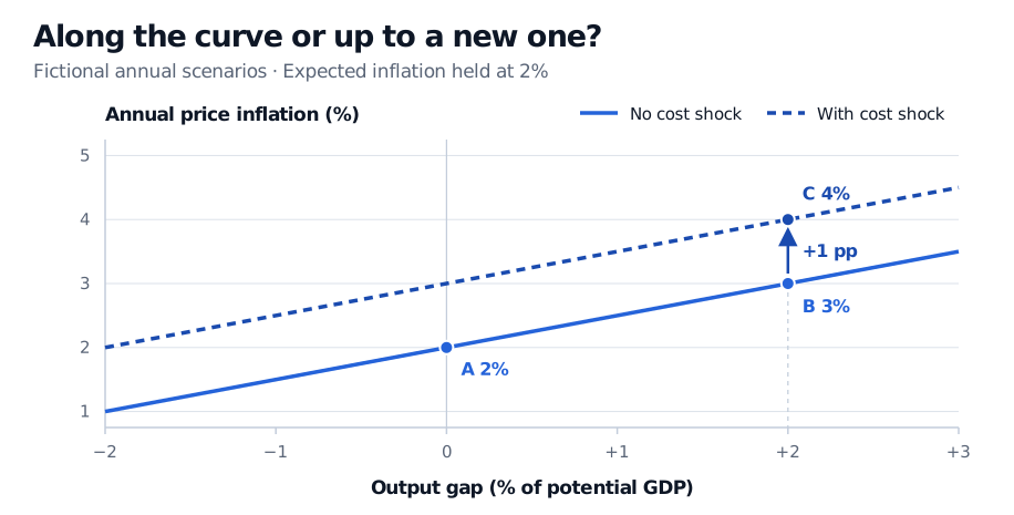
The move from A to B isolates a wider output gap. The move from B to C isolates a one-percentage-point cost shock at the same gap.
Why a fitted slope can mislead
A regression through all observed inflation and output-gap pairs can look flat even when the conditional curve slopes up. For example, a central bank that tightens in response to a cost shock can restrain demand while inflation remains high. Those observations pair higher inflation with a smaller output gap. Researchers look for variation in demand that can be separated from cost shocks and policy responses. Estimates also depend on the sample and how slack is measured. Some regional studies find a steeper curve in very tight labour markets than in normal conditions. McLeay and Tenreyro (2019), Sections 1–2, Smith, Timmermann and Wright (2024), Results
The SelfMadeQuant Endogeneity and Instrumental Variables lesson explains how a shock can bias a fitted slope and what makes an instrument credible. The preview is public. The full lesson requires membership.
Expectations can adjust, too. A credible inflation target can help anchor longer-run expectations even when near-term expectations rise. In the simplified model, if a higher inflation rate becomes fully expected and the supply shock has passed, implies . Permanently higher inflation therefore buys no permanent increase in output relative to potential in this framework. The short-run slope alone cannot tell a policymaker how output and inflation will respond to a rate decision. Friedman (1968), Section I, Jørgensen and Lansing (2021), “Improved anchoring”
Sources
- A. W. Phillips (1958). The Relation Between Unemployment and the Rate of Change of Money Wage Rates in the United Kingdom, 1861–1957.
- Milton Friedman (1968). The Role of Monetary Policy.
- Michael McLeay and Silvana Tenreyro (2019). Optimal Inflation and the Identification of the Phillips Curve.
- Peter Lihn Jørgensen and Kevin J. Lansing (2021). Federal Reserve Bank of San Francisco. Return of the Original Phillips Curve.
- Francesco Furlanetto and Antoine Lepetit (2024). Federal Reserve Board. The Slope of the Phillips Curve.
- Simon C. Smith, Allan Timmermann and Jonathan H. Wright (2024). Federal Reserve Board. Nonlinear Phillips Curves.