Okun's Law is the empirical tendency for the unemployment rate to rise when real GDP grows below its normal pace and to fall when growth exceeds that pace. A macro analyst can use it to check whether a growth scenario and an unemployment forecast tell a consistent story. Arthur Okun originally studied both changes and gaps using US real GNP. Okun (1962)
Why positive growth can come with rising unemployment
A simple difference specification centres real GDP growth on an estimated benchmark . In this model, is the growth rate at which the predicted change in unemployment is zero. Put both growth rates on the same horizon and express them in percent. Then their difference is in percentage points (pp), as is the predicted change in unemployment. Knotek (2007), Section I
Suppose a fictional annual scenario has normal growth, actual growth and a slope of pp of unemployment-rate change per pp of real GDP growth above normal. The one-point shortfall gives
An initial unemployment rate of therefore gives a predicted rate of one year later. Output still grew. It just grew more slowly than the model's benchmark for stable unemployment.
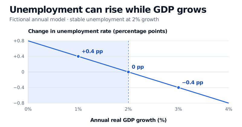
The line shows model predictions under the stipulated slope. The shaded region marks growth below the 2% benchmark.
The gap version compares levels
The gap specification relates the unemployment rate relative to its estimated normal level to the output gap . Define as actual real GDP minus potential output, expressed as a percentage of potential output. Then a simple fitted relationship is
A negative output gap goes with a positive predicted unemployment gap. An economy can grow faster than normal and still produce below potential. In that case the difference model can predict falling unemployment while the gap model still points to unemployment above its benchmark. Each specification has its own fitted slope. Knotek (2007), Section I and appendix
When the forecast misses
Firms may cut hours before reducing headcount, so unemployment can respond to GDP with a lag. A shift in labour-force participation can also change unemployment for a given level of employment. US rolling estimates have varied across sample windows, and estimates differ across countries. The slope measures observed co-movement. Estimating the unemployment effect of a particular policy requires isolating that policy's effect from other forces moving output and unemployment. Knotek (2007), Section II, Ball, Leigh and Loungani (2017), Sections 1, 4 and 5
Check the data vintage before interpreting a large forecast error as a change in the relationship. After the Great Recession, downward revisions to US real GDP per working-age person made the rise in unemployment look more consistent with historical experience. A backtest should fit its growth benchmark and slope using only the data available at each forecast date. The SelfMadeQuant Point-in-Time Data lesson covers selecting the eligible revision and auditing that cutoff. The preview is public and the full lesson requires membership. Daly, Fernald, Jordà and Nechio (2014)
Sources
- Arthur M. Okun (1962). Potential GNP: Its Measurement and Significance.
- Edward S. Knotek II (2007). Federal Reserve Bank of Kansas City. How Useful Is Okun's Law?.
- Laurence Ball, Daniel Leigh and Prakash Loungani (2017). Okun's Law: Fit at 50?.
- Mary C. Daly, John Fernald, Òscar Jordà and Fernanda Nechio (2014). Federal Reserve Bank of San Francisco. Interpreting Deviations from Okun’s Law.