Count ordered selections without repetition, distinguish them from subsets and repeated draws, and see when order matters in quant research and financial paths.
Permutation
A permutation is an ordering of distinct objects. Arranging all n objects gives n! possibilities; choosing and ordering only k of them, without repetition, gives a k-permutation. The distinction matters whenever a research ranking, execution priority or assignment to different roles is part of the outcome.
Three priorities, five candidates
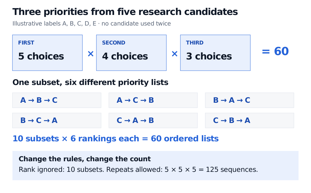
A hypothetical quant team has five candidate signals, labelled A through E, and capacity to investigate three. Its research plan names a first, second and third priority, with no signal appearing twice. A–B–C and B–A–C are different plans: they allocate the earliest research slot differently.
There are five choices for first priority. Once it is chosen, four remain for second; then three remain for third. The number of plans is
P(5,3)=5×4×3=60.
This counts possible priority lists, not profitable signals, independent experiments or distinct trading strategies. If all three signals eventually receive the same treatment, the priority lists may lead to the same final research output. Count outcomes at the level the decision actually distinguishes.
Five distinct research candidates fill first, second and third priority with five, four and three choices, producing 60 lists. The subset A, B, C has six rankings. Ignoring rank gives 10 subsets; allowing repeats gives 125 sequences.
Original illustrative research-planning example. Each selected signal occupies one priority slot. The six displayed lists share the same subset; the other subsets are not shown.
Why the factorial ratio works
For integers 0≤k≤n, count the available labels in each successive slot:
P(n,k)=n(n−1)⋯(n−k+1)=(n−k)!n!.
The factorial ratio cancels the unused tail of the product. It is also written nPk or (n)k, although the latter notation needs context because conventions vary.
For k=n, this becomes n!: all objects are arranged. For k=0, there is one empty list, so P(n,0)=1, including P(0,0)=1. Selecting more than n distinct labels without replacement is impossible; its count is zero, rather than a factorial of a negative integer.
If priority is irrelevant, divide by k!. Every selected set of k distinct objects has exactly that many rankings. The binomial coefficient counts these unordered selections:
(kn)=k!P(n,k).
Our team therefore has 60/3!=10 possible three-signal subsets, each associated with six priority lists. Choosing which signals to study and ranking the chosen signals answer different questions.
Two meanings of “repetition”
Allowing a label to be selected again changes the research example into a different experiment. If any of five labels can occupy each of three slots, including A–A–A, there are 53=125 ordered sequences. Each slot retains five choices. The no-replacement formula does not apply.
Rearranging a fixed collection containing identical labels is another problem. For example, the fixed labels A, A, B have only three distinguishable arrangements: AAB, ABA and BAA. Temporarily distinguishing the two A labels gives 3! arrangements, but swapping those labels changes nothing visible, so divide by 2!. More generally, a fixed collection of n objects with identical-label multiplicities m1,…,mj has
m1!⋯mj!n!,m1+⋯+mj=n
distinguishable arrangements. This division assumes objects within each group are truly interchangeable for the question being asked. Two trades with the same ticker can still be distinct if their timestamps, sizes or prices matter.
Counting is not a probability model
The 60 priority lists form a finite sample space, but their count alone supplies no probabilities. If the team draws uniformly from the remaining labels at each slot, a specified list has probability (1/5)(1/4)(1/3)=1/60, and a specified subset has probability 6/60=1/10. If research priorities favour familiar signals, those uniform probabilities are unjustified. Berkeley's Data 140 text develops the relationship between uniformly random orderings and unordered samples.
Likewise, shuffling historical observations for a statistical test requires a null model that permits the proposed rearrangements. Merely knowing how many permutations exist does not justify treating time-series observations as freely exchangeable.
In financial paths, ask what the order changes. With no intervening flows and a fixed fully invested position, terminal wealth W0∏t=1n(1+rt) is unchanged when the same simple returns are reordered. Intermediate wealth, barrier crossings and decisions triggered along the path can change. Permutation counting identifies possible arrangements; the payoff or decision rule determines whether those arrangements matter economically.
For a fuller derivation, including partitions and worked counting problems, see Counting and Combinatorics. The full supporting Library lesson requires membership; a public preview provides its outline.
Sources
Joseph K. Blitzstein and Jessica Hwang, Introduction to Probability, 2nd edition, §1.4.1: multiplication rule, Theorems 1.4.7–1.4.8 on sampling with and without replacement, and Example 1.4.9 on permutations and factorials.