How MARS learns nonlinear responses using paired hinges, adaptive knots and pruning; a worked predictor separates additive effects, interactions and smoothing.
Multivariate adaptive regression splines
Multivariate adaptive regression splines (MARS) is a regression method that builds a response surface from data-selected spline basis functions and their products. For a quant modelling a nonlinear relationship between trading cost and order size, it offers interpretable changes in slope without requiring a single straight-line response across the whole size range.
“Multivariate” refers here to using several predictors. MARS does not inherently make the model autoregressive: lagged observations become inputs only if the researcher supplies them.
A hinge changes the slope
In the first-degree hinge formulation, a knot t gives two building blocks:
h+(x;t)=max(0,x−t),h−(x;t)=max(0,t−x).
Both are continuous. Each is zero on one side of the knot and linear on the other. A predictor adds weighted basis functions:
f^(x)=β0+m=1∑MβmBm(x).
A basis function Bm can be one hinge or a product of hinges on distinct predictors. Conditional on the selected basis, the coefficients can be estimated by ordinary least squares. Selecting that basis is itself an adaptive modelling step. Friedman (1991), §3.4, describes the first-degree construction.
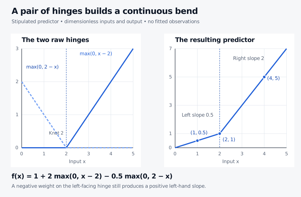
Consider this stipulated predictor, with dimensionless input and output:
f(x)=1+2max(0,x−2)−0.5max(0,2−x).
The knot and coefficients are given for illustration; no data have been fitted. Below the knot, only the left-facing hinge contributes. Above it, only the right-facing hinge contributes. Expanding each branch gives
f(x)={0.5x,2x−3,x≤2,x>2.
Input x
Right hinge
Left hinge
Prediction f(x)
1
0
1
0.5
2
0
0
1
4
2
0
5
The two branches meet at one, but the slope changes from 0.5 to 2. The left hinge's coefficient is negative; the left-hand slope is positive, because increasing x makes 2−x smaller.
Two raw hinges are nonnegative and meet at knot 2. Their weighted sum plus intercept gives f(1) = 0.5, f(2) = 1 and f(4) = 5. The predictor has slope 0.5 before the knot and 2 after it.
Original dimensionless illustration of a stipulated predictor, with no fitted observations. The raw left-facing hinge falls as x increases; its negative coefficient makes its contribution rise.
Grow a basis, then prune it
The regression version has two selection stages:
Forward construction. Start with an intercept. Search over eligible parent basis functions, predictors and candidate knots. Add the pair Bm(x)h+(xj;t) and Bm(x)h−(xj;t) giving the best improvement in squared-error fit, retaining the parent and refitting coefficients. Limits on basis size and interaction order constrain the search.
Backward pruning. Remove basis terms and refit, producing a sequence of smaller models. Select a model using a complexity-adjusted criterion, classically a modified generalised cross-validation criterion. The selected model need not retain every forward-stage hinge pair.
This is an intentionally generous construction followed by simplification; the forward fit alone is vulnerable to overfitting. The SAS ADAPTIVEREG fitting-algorithm description, under Forward Selection and Backward Selection, sets out these stages. It is a description of the method, not a requirement to use that software.
Products create interactions
Using only univariate hinge terms makes the response additive, relating MARS to a generalised additive model. Products allow one predictor's effect to depend on another. For example,
B(x,z)=max(0,x−2)max(0,z−1).
Increasing x from two to three changes this basis term by zero when z=1, but by one when z=2. That dependence on z is the interaction. In a trading-cost application, it could represent a size effect that changes with a liquidity measure; interpreting it as a causal effect would require a separate research design.
“First-degree” describes each hinge factor. With products, the full surface is piecewise multilinear, rather than generally piecewise linear jointly in all inputs. A two-factor product can contain an xz term even though each one-variable slice is piecewise linear.
Smoothness is a separate choice. The hinge predictor above has a kink. Friedman's original paper, §3.7, also constructs a smoothed piecewise cubic basis around the selected knots, giving continuous first derivatives, but not generally continuous second derivatives. That refinement is different from the unsmoothed hinge example shown here. A claim that every MARS fit has smooth derivatives would therefore be misleading.
Keep adaptation inside the training window
Knots, retained terms, coefficients and preprocessing must be learned within each training fold. Use validation folds to compare model choices such as maximum basis size and interaction order; do not choose knots once on the full dataset and then call the resulting scores cross-validation. The general separation of fitting from held-out data is explained in scikit-learn's data-leakage guidance.
For financial forecasting, apply that separation chronologically: inputs must have been available at the forecast time, and training labels must be observable before the evaluation window. Overlapping return horizons may require an additional gap between training and validation. A favourable pruning criterion is not a substitute for a later untouched test period.
The example's right branch continues as 2x−3 outside the illustrated range. That is the formula's extrapolation rule, not evidence that a real cost relationship remains linear there. Likewise, an adaptively chosen knot need not identify an economic regime boundary.