A GAM adds smooth predictor effects on a link scale. See how response links, centering, smoothing penalties and interactions shape its interpretation.
Generalised additive model
A generalised additive model (GAM) models a response through a sum of smooth predictor functions, linked to its conditional mean. For a quant modelling trade arrivals or a nonlinear risk signal, it permits curved relationships while keeping individual model contributions visible.
Here g is the link, ηi is the additive predictor, and each fj is a smooth function learned from data. A function can curve, flatten or reverse slope. Some predictors can retain ordinary linear terms. The response family supplies distributional assumptions beyond this mean equation. Hastie and Tibshirani's original paper develops the additive construction and iterative estimation.
Add on the link scale
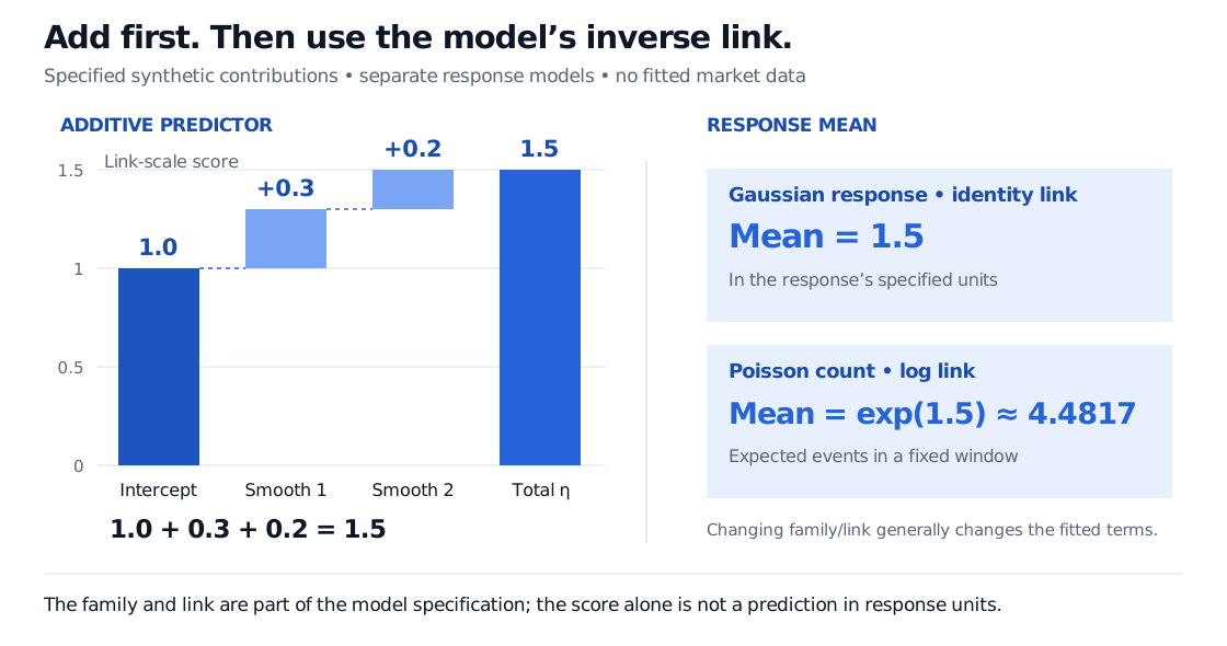
Suppose the intercept is 1 and two smooths contribute 0.3 and 0.2 at a particular predictor combination. Then
η=1+0.3+0.2=1.5.
That score becomes a response mean only after specifying a family and link:
Separate illustrative specification
Conditional mean at this score
Gaussian response with identity link
μ=η=1.5 response units
Poisson trade count with log link, fixed observation window
μ=eη=e1.5≈4.4817 expected trades
These are two specified models, each assigned the same contributions for illustration. Changing the family or link and refitting data generally changes the estimated functions too. The fractional Poisson mean is an expected count, not a possible realised trade count. The R family documentation distinguishes family and link choices.
Synthetic GAM waterfall: intercept 1, smooth contribution 0.3 and smooth contribution 0.2 give a link-scale score of 1.5. Separate Gaussian identity-link and Poisson log-link specifications give means of 1.5 response units and 4.4817 expected events per window.
Original stipulated example, not a fitted dataset. Additivity describes the predictor; the inverse link determines how that predictor becomes a conditional mean. The two response specifications need not produce the same fitted terms when estimated.
With a log link, a 0.2 increase in one smooth, holding the other terms fixed, multiplies the mean by e0.2≈1.2214. It does not add 0.2 trades. The absolute change in the mean depends on the starting mean even when the predictor is additive. Also, the model concerns the log of the conditional mean, not the conditional mean of logged observations.
Smooth does not mean unconstrained
A common implementation represents each curve with spline basis functions and fits their coefficients jointly. One penalised-likelihood formulation minimises
−ℓ(θ)+21j∑λjJ(fj),
where ℓ is the response log likelihood, θ collects the coefficients, J measures roughness, and λj≥0 controls the fit–smoothness trade-off. For a suitable twice-differentiable univariate curve, a familiar penalty is J(fj)=∫{fj′′(u)}2du.
Larger penalties discourage wiggles; they do not necessarily eliminate an entire term, because some function components can escape a particular penalty. A sufficiently rich basis still needs regularisation against overfitting; an undersized basis can prevent useful curvature even with a small penalty. Smoothing parameters may be selected using criteria such as REML or generalised cross-validation. These are modelling choices, not guarantees of forecast quality. Wood's fitting documentation explains this construction and its limits.
The curves are not separate regressions of the response on each predictor. In backfitting, each curve is updated using residuals after the current contributions of the others have been removed; updates repeat. Penalised spline methods likewise estimate a combined model. This matters when predictors overlap in what they explain. Hastie and Tibshirani, §7.
Why component plots are centred
Without a constraint, adding a constant to a smooth and subtracting it from the intercept leaves every prediction unchanged. For the example, replacing the intercept 1 by 0.9 and the first contribution 0.3 by 0.4 still gives η=1.5.
A common identification convention imposes
i=1∑nfj(xij)=0
on each ordinary smooth over the training observations. The intercept then carries the overall level on the link scale. This is a centering convention, not evidence that a zero crossing is an economic threshold. Some smooth types require different constraints. Wood's identifiability documentation states these exceptions.
A component curve usually shows a centred contribution on the linear-predictor scale, rather than the predicted response or its stand-alone expectation. Exponentiating one component in a multivariable log-link model gives a multiplicative factor, not the complete mean. The plotting documentation describes the scale and uncertainty conventions.
What the additive restriction leaves out
The univariate sum above contains no interaction: the change in f1 does not depend on the value of the second predictor. If momentum's contribution on the link scale changes with volatility, the model may need an explicit smooth interaction such as f12(x1,x2). GAM frameworks can include such multivariable terms, with suitable constraints and penalties. They remain structured models, though a one-dimensional curve no longer describes the whole effect of either interacting variable. Wood's model specification guide distinguishes main effects and interactions.
Smooth terms can also mimic one another when predictors are related. This concurvity can make the allocation between component curves unstable even when aggregate predictions look reasonable. Centering alone does not fix it. Wood's concurvity documentation explains this generalisation of collinearity.
A visible curve describes the fitted conditional association under the chosen model. It does not establish what would happen if a trader intervened on that predictor: confounding, selection and reverse causation require a separate causal argument.