Choose between nominal class logits and ordered cumulative thresholds, recover category probabilities, and interpret reference classes and proportional odds with an explicit sign convention.
Multinomial and ordinal logistic regression
Multinomial logistic regression models probabilities of mutually exclusive categories with no imposed order. Ordinal logistic regression uses an outcome's ranking; its common cumulative-logit form models the probability of being at or below each category boundary. A quant forecasting an execution venue faces nominal labels; a quant forecasting low, medium or high credit stress has ordered labels. Choosing the response model determines which relationships the fitted probabilities must obey.
Both extend binary logistic regression. Assigning category codes 1, 2 and 3 does not establish equal distances between categories, or make a continuous-outcome regression appropriate. An ordinal model uses the ranking without assuming those distances.
Nominal outcomes: one relative score per class
For classes k=1,…,K and predictors x, define linear scores zk=αk+x⊤βk. Multinomial logit applies softmax:
pk(x)=P(Y=k∣x)=∑r=1Kezrezk.
These probabilities are positive and sum to one. A single observation has one categorical outcome; the multinomial distribution describes category counts over repeated independent observations with common probabilities. Regression allows those probabilities to depend on predictors.
Only score differences are identified: adding the same quantity to every score leaves softmax unchanged. A reference-class convention sets z1=0, including that class's intercept and coefficients. Then
logp1(x)pk(x)=αk+x⊤βk,k=2,…,K.
Other constraints or penalised symmetric parameterisations are possible. State the convention before interpreting a coefficient: it describes a log probability ratio against a reference category, not a direct percentage-point effect. The scikit-learn multinomial formulation explains its symmetric parameterisation and the unpenalised non-uniqueness.
For numerical computation, subtract m=maxrzr before exponentiating: use ezk−m/∑rezr−m. This leaves probabilities unchanged and prevents overflow from large positive scores. Independently fitting binary “class versus all others” models is a different construction; the raw binary probabilities need not sum to one.
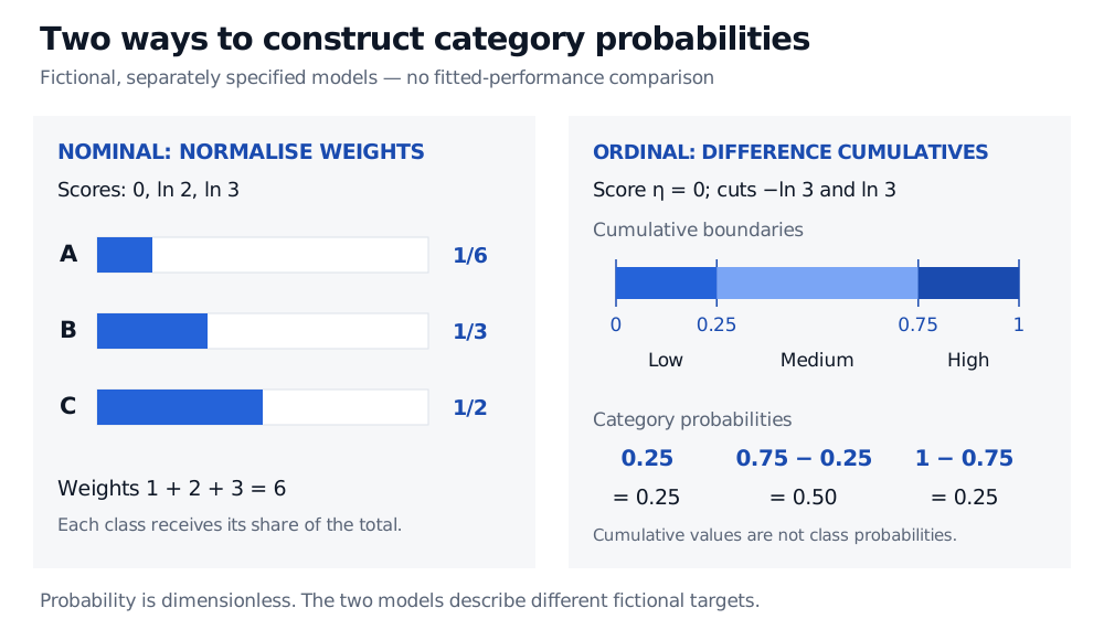
Fictional nominal example. Suppose three execution-venue classes A, B and C have stipulated scores 0,log2,log3. Their exponentiated weights are 1,2,3, so the probabilities are 1/6,1/3,1/2. C is the most likely single label; its probability is only one half. These numbers are specified for illustration, not estimates of venue selection or execution quality.
Ordered outcomes: cumulative boundaries, then differences
Now consider a separate model for low, medium and high stress, coded in increasing order. Write η=x⊤β and impose ordered cutpoints c1<⋯<cK−1. This article uses
Fj(x)=P(Y≤j∣x)=σ(cj−η),σ(u)=1+e−u1,j=1,…,K−1.
The cut-minus-score sign matches McCullagh's §2.1 cumulative-logit formulation. A larger η lowers every cumulative probability, shifting the distribution toward higher categories. Software can use the opposite sign or reverse the category order, so a coefficient's direction has meaning only after both conventions are known.
Recover the category probabilities by taking differences:
p1=F1,pj=Fj−Fj−1(2≤j≤K−1),pK=1−FK−1.
Ordered cuts make these probabilities nonnegative. Cumulative probabilities are nested events, not separate class probabilities: adding them is not a valid normalisation. The statsmodels model description gives the equivalent interval-probability construction.
Fictional ordinal example. Set η=0, c1=−log3 and c2=log3. Then F1=1/4 and F2=3/4. Low, medium and high probabilities are therefore 1/4,1/2,1/4: medium is 3/4−1/4, not 3/4.
Separate fictional models. Nominal logits 0, ln 2 and ln 3 give A, B and C probabilities 1/6, 1/3 and 1/2. Ordinal cumulative probabilities 0.25 and 0.75 give low, medium and high probabilities 0.25, 0.50 and 0.25.
Separate stipulated models illustrate two probability constructions. Their different outputs are not a comparison of fitted performance.
What proportional odds assumes
In this cumulative model,
log1−Fj(x)Fj(x)=cj−x⊤β.
The same slope vector appears at every boundary. A one-unit rise in predictor xr, holding other predictors fixed, multiplies the cumulative odds of Y≤j by e−βr for everyj. The reciprocal odds of being above the boundary are multiplied by eβr. This is the proportional-odds restriction: a common odds ratio, not equal changes in category probabilities.
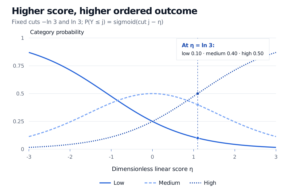
With the example's cuts fixed, increasing η from zero to log3 changes the cumulative probabilities to 0.10 and 0.50, hence category probabilities to 0.10,0.40,0.50. Both cumulative odds fall by a factor of three, although category probabilities move by different amounts. A middle category need not move monotonically as the score rises.
Ordered-logit probabilities as the dimensionless score eta rises from minus 3 to 3 with cuts fixed at minus ln 3 and ln 3. Low probability decreases, high increases and medium peaks at eta zero. At eta ln 3, probabilities are 0.10, 0.40 and 0.50.
A higher score shifts probability toward higher ordered categories under the stated cut-minus-score convention. The middle category can first gain and then lose probability.
The cutpoints already supply intercept-like locations. Adding a free common intercept to η while estimating all cuts freely is unidentified: shifting that intercept and all cuts by the same amount changes nothing. One conventional specification omits the common intercept and fixes the logistic error scale; statsmodels' Notes spell out the constant-term problem. Cuts are boundaries on the model's score scale, not observed numerical distances between rating grades.
Choosing and checking the response model
Use nominal logit when the labels have no meaningful ordering, or when its separate class effects suit the problem. It can also model ordered labels while leaving their order unused. Use cumulative ordinal logit when the ordering matters and common boundary slopes are defensible. Ordered labels alone do not establish proportional odds: a predictor could strongly distinguish high stress from the rest while barely distinguishing low stress from the rest. Boundary-specific diagnostics and more flexible ordinal specifications can reveal or accommodate that mismatch, provided cumulative probabilities remain ordered.
Both models can be fitted by maximum likelihood, using the probability of each observed category; regularisation changes the fitting objective. Compare fitted alternatives using the same held-out target and information set. In financial data, preserve observation timing and test probability calibration by class and relevant period rather than assuming that a normalised output is an accurate probability. A most-likely category also need not be the best decision when misclassification costs differ.