A mispricing factor model explains asset returns using factors built from stock characteristics interpreted as proxies for relative mispricing. Instead of treating each anomaly as a separate factor, it combines several signals into composite rankings and trades the extremes. For a quant evaluating a strategy, this creates a benchmark: apparently stock-specific alpha may partly reflect exposure to a common anomaly portfolio.
The best-known example is the four-factor model of Stambaugh and Yuan, published in 2017. Its factors are market excess return, a specially constructed size factor, and two composite mispricing factors, MGMT and PERF. A “mispricing” label does not mean the model observes fair value or proves irrational pricing. Stambaugh and Yuan, introduction.
Two composites, not eleven separate bets
The original groups are:
| Composite | Anomaly inputs |
|---|---|
| MGMT | Net stock issues; composite equity issues; accruals; net operating assets; asset growth; investment-to-assets. |
| PERF | Distress; O-score; momentum; gross profitability; return on assets. |
The groups reflect similarities in anomaly returns, rather than an assumption that all eleven signals describe one mechanism. The first group is more directly related to management decisions; the second to firm performance. Each composite averages the available rankings within its group. Author manuscript, §3.1.
Orientation comes before averaging. A high rank must consistently mean more overpriced by the proxy: raw profitability and raw accruals cannot simply be ranked in the same direction. Rankings are formed before the returns being measured. The manuscript uses end-of-month information for month , with source-specific accounting lags and missing-data requirements: at least three available anomalies per stock within a cluster, and at least 30 stocks for an anomaly to enter. Author manuscript, §3.1 and Appendix A1. A reproduction using subsequently revised or unreleased information introduces look-ahead bias.
The published construction independently sorts size at the NYSE median and each composite at the combined-universe 20th and 80th percentiles. Stocks priced below five US dollars are excluded. Within each size group, value-weighted low-score portfolios are bought and high-score portfolios sold; the two size-specific spreads are averaged. Its size factor instead uses stocks in the middle of both composite sorts, taking small minus big. It is therefore not interchangeable with an arbitrary standard SMB series. Published paper, §2.1–2.2.
A six-stock miniature
This fictional example isolates rank aggregation and payoff arithmetic. It uses two signals, no size split and equal stock weights; it does not reproduce the eleven-anomaly benchmark or either named factor.
At the decision date, both signals have already been oriented so higher means more overpriced:
| Stock | Signal 1 rank | Signal 2 rank | Mean rank | Signed weight | Next-period simple return |
|---|---|---|---|---|---|
| A | 1 | 2 | 1.5 | +0.5 | +2% |
| B | 2 | 1 | 1.5 | +0.5 | +1% |
| C | 3 | 4 | 3.5 | 0 | 0% |
| D | 4 | 3 | 3.5 | 0 | 0% |
| E | 5 | 6 | 5.5 | −0.5 | −1% |
| F | 6 | 5 | 5.5 | −0.5 | 0% |
For A, the score is . Buy A and B and short E and F. Each leg has notional 1, so gross exposure is 2 and net exposure is 0. Equal composite scores cause no boundary ambiguity here because each tied pair is kept together; a larger implementation needs an explicit tie rule.
The subsequent long-basket return is . The basket that was shorted returns . Thus the long-short portfolio payoff is
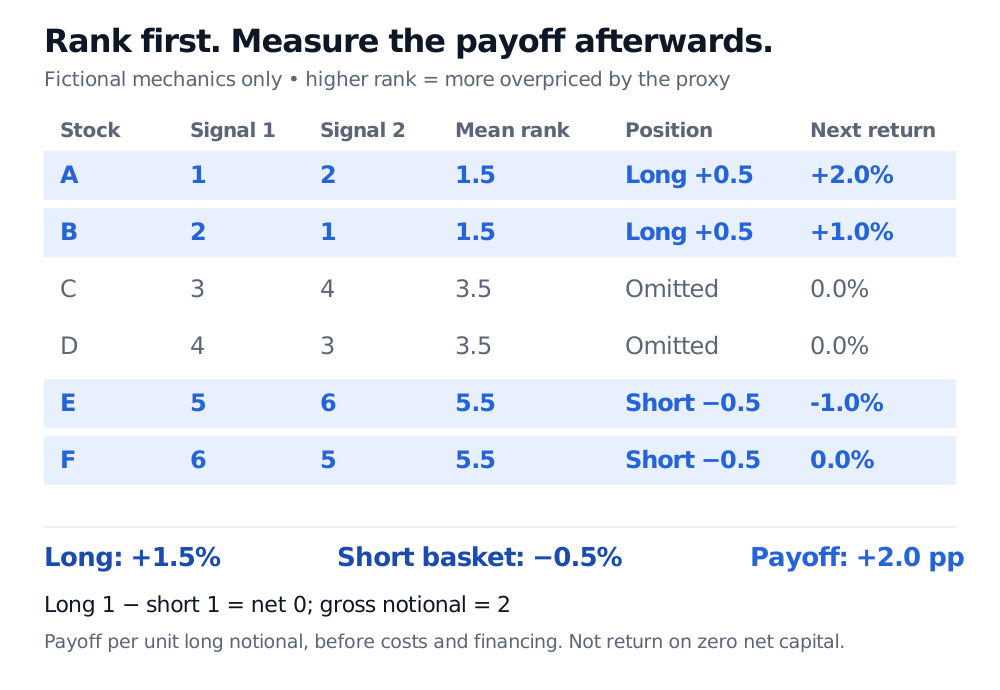
A reduced two-signal example separates the ranking decision from next-period returns; it is not a replication of MGMT or PERF.
That is a 2 percentage point payoff per unit long notional, before borrow fees, trading costs and financing. Dividing by gross notional gives 1%; dividing by zero net notional is undefined. Return on an investor's committed capital requires a separate capital convention. Dollar neutrality also does not automatically make the basket beta-neutral.
From a score to an explanatory model
A stock's composite score selects its portfolio membership. It is not the stock's regression loading. Once the four factor return series exist, estimate factor exposures using, for example,
A loading describes co-movement with a factor; the score is an input to constructing that factor. A high composite score is neither a dollar estimate of overvaluation nor a promised negative next-period return.
The authors report stronger historical anomaly accommodation than the comparison models they tested, and sentiment predictability consistent with a mispricing interpretation. The tests use historical US data ending in 2013; later periods and other universes require fresh validation. Published introduction and §2. These findings are not causal identification of investor irrationality or a guarantee of a future factor premium. Construction choices, shorting constraints and costs matter when carrying a research benchmark into a tradable strategy. September 2016 abstract.
For the surrounding signal vocabulary, Quantitative Factors compares value, quality and momentum and discusses standardising signals before combining them. The public page is a preview; the full lesson requires membership.
Sources
- Stambaugh, R. F. and Yuan, Y. (2017). Mispricing Factors, Review of Financial Studies, 30(4), 1270–1315. Introduction and §2 explain the model and portfolio construction.
- Stambaugh, R. F. and Yuan, Y. January 14, 2016 author manuscript, §3 and Appendix A1, for the cluster inputs, orientation, timing and eligibility rules.
- Stambaugh, R. F. and Yuan, Y. September 17, 2016 manuscript, title page and abstract, for the forthcoming-paper version and summary of historical findings.