Frozen base weights, trainable low-rank updates, a checked parameter-count example and the limits of LoRA memory savings.
Low-rank adaptation
Low-rank adaptation (LoRA) adapts a pretrained neural network by freezing selected weight matrices and learning a low-rank additive update to them. A quant team could use it to adapt a language model to labelled earnings-call passages while training and saving far fewer task-specific parameters. Whether those labels improve on a simpler classifier remains a held-out measurement question.
LoRA is a form of parameter-efficient fine-tuning: training changes the model, but the optimiser updates only a small set of additional weights. The original LoRA paper by Hu et al., §4, introduces the factorised update and shows how it can be merged into the original weights.
Keep the matrix, constrain the change
Use column-vector inputs. A frozen linear layer has W0∈Rd×k, input x∈Rk and output in Rd. Standard LoRA writes
h=W0x+ΔWx,ΔW=rαBA,A∈Rr×k,B∈Rd×r.
The positive integer r is the chosen adapter rank, and α controls the update's scale. Here, standard LoRA means the original α/r scaling; some variants use other conventions. Biases and other trainable modules are excluded from this calculation.
The matrix rank of ΔW is at mostr, because its output lies in the span of the r columns of B. Training learns both factors. It does not require either factor to be orthogonal, and does not obtain them by truncating the pretrained matrix's singular values.
In particular, W0+ΔW can remain full rank. LoRA constrains the change, unlike replacing the entire layer with a low-rank approximation.
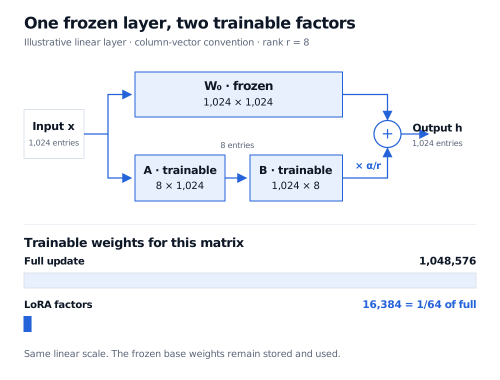
Column-vector input x follows two paths: a frozen 1024 by 1024 W0 and trainable A of shape 8 by 1024 followed by B of shape 1024 by 8, scaled by alpha over r and added to the frozen output. The adapter has 16,384 trainable weights versus 1,048,576 for the full matrix, a fraction of 1 over 64.
Illustrative single-layer LoRA, with rank 8. The bars compare trainable scalar weights on the same linear scale; the frozen base matrix still has to be stored and used.
What the 64-fold reduction counts
For a frozen 1024×1024 weight matrix and r=8, the two factors contain
A8×1024+B1024×8=16,384
trainable scalar weights. Updating every entry of the original matrix would involve 1,048,576 weights, so the adapter's count is 1/64=1.5625% of that full-matrix count.
This is 64 times fewer trainable weights for this matrix. It does not establish a 64-fold reduction in whole-model training memory or runtime. The frozen weights remain present, activations still occupy memory, and gradients must still propagate through the network to train the adapters. Training memory also depends on optimiser state, precision, batch size and sequence length. Additional trainable heads or biases change the count too.
The current PEFT LoRA documentation distinguishes the rank, target modules, scaling, biases and separately saved trainable modules. A parameter ratio for one matrix cannot substitute for measuring the configured training job.
A rank-one change you can multiply by hand
Consider a separate, deliberately tiny layer with d=k=2, r=1 and α=1. The scaling is therefore α/r=1. Suppose the learned factors are
B=(12),A=(34).
Their update is
ΔW=BA=(3648).
The second row is twice the first. For any input, the extra output lies along (1,2)⊤. For example, x=(2,−1)⊤ gives Ax=2, followed by B(Ax)=(2,4)⊤. Multiplying the displayed update by x gives the same answer.
If W0=I2, then W0+ΔW has rows (4,4) and (6,9) and determinant 12. The adapted matrix has rank two even though its update has rank one. This tiny example teaches the constraint; its two factors contain four scalars, so it offers no parameter saving over a four-entry full matrix.
A zero update can still start learning
The original paper initialises A randomly and B at zero. PEFT's documented default uses a random Kaiming-uniform A and zero B. In either case, the adapter initially adds nothing.
Zero initial output does not mean every learning gradient is zero. Write s=α/r and let G be the loss gradient with respect to the effective weight matrix. For the task loss through this layer,
∇BL=sGA⊤,∇AL=sB⊤G.
At B=0, the gradient for A is zero, while the gradient for B can be nonzero when A is nonzero. Nonzero A alone does not guarantee a nonzero B gradient: it also depends on G. Initialising both factors at zero makes both task-loss gradients zero. These statements concern the task loss, separately from any weight-decay update.
Using the saving in financial text research
Choose the target matrices, rank, scaling and stopping rule using training and validation data. A smaller adapter can still overfit; fewer trained weights do not prove that the task needs only a low-rank change. Keep a later test period untouched, and check whether the base model's pretraining or the adaptation corpus introduces look-ahead bias.
For standard linear LoRA at inference, one can form Wmerged=W0+(α/r)BA. The merged layer uses the usual matrix multiplication, without a separate adapter branch. This does not shrink the base model's dimensions. Alternatively, keep the factors separate when swapping task adapters; then the extra branch remains part of the computation.
QLoRA adds another memory-saving mechanism: the QLoRA paper describes learning low-rank adapters through a frozen, four-bit quantised base model. Low-rank updates and reduced-precision storage address different parts of the memory budget. LoRA itself does not require four-bit weights.
The Transformers lesson develops the fine-tuning and held-out validation context for financial text. Kernel, Image, and the Rank-Nullity Theorem explains why a map's image limits its output directions. Both have public previews; full lessons require membership.