Read cumulative-share inequality from a Lorenz curve, calculate Gini by areas and pairwise differences, and distinguish sample normalisation, weighting and risk.
Lorenz curve and Gini coefficient
A Lorenz curve plots the cumulative share of a nonnegative quantity against the cumulative share of units, ranked from the smallest quantity to the largest. The Gini coefficient summarises its distance below equal allocation: zero means equal amounts, and larger values mean greater relative inequality under the same convention. For a quant examining loan sizes or account balances, the pair shows how much of the total sits with the larger units; it does not establish how risky those units are.
The standard construction requires nonnegative values and a strictly positive aggregate. Individual zeros are allowed. A zero aggregate leaves the shares undefined; negative net wealth or trading profit needs separate treatment rather than the usual zero-to-one interpretation.
Count accounts, then accumulate dollars
Consider four fictional loan accounts with exposures of USD 1 million, USD 2 million, USD 3 million and USD 4 million. Each account has equal weight as a unit; the exposures total USD 10 million.
Smallest accounts included
Share of accounts
Cumulative exposure
Share of exposure
None
0%
USD 0m
0%
First
25%
USD 1m
10%
First two
50%
USD 3m
30%
First three
75%
USD 6m
60%
All four
100%
USD 10m
100%
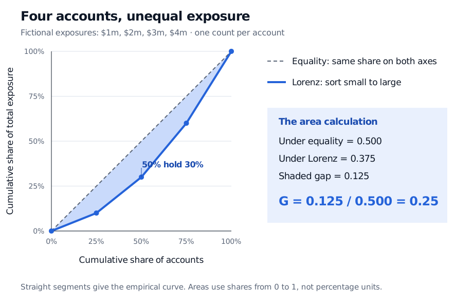
The bottom half of accounts holds 30% of exposure; the largest account holds 40%. Plot the two share columns, include the origin and join consecutive points with straight segments. Equal exposures would give the diagonal: the bottom half would hold exactly half of the total. This cumulative-share construction is the one described by the ONS methodology.
Fictional exposures of 1, 2, 3 and 4 million dollars give cumulative exposure shares 0, 10, 30, 60 and 100 percent at account shares 0, 25, 50, 75 and 100 percent. Lorenz area is 0.375; the gap below equality is 0.125; Gini is 0.25.
Original fictional account exposures. Each account contributes one unit to the horizontal axis. The shaded area is the gap below equality; all area calculations use shares from zero to one.
The horizontal axis counts accounts, not dollars of exposure. Choosing borrowers instead would first require aggregating each borrower's accounts. Splitting one loan into several account records can change the answer without changing the lender's economic exposure. Define the unit before comparing two Ginis.
An area ratio, with a check from every pair
Write the curve as L(p), where p is the cumulative fraction of units. The equality triangle has area 1/2, so
G=1/21/2−∫01L(p)dp=1−2∫01L(p)dp.
For the straight empirical segments, the trapezoidal rule gives the area exactly. With pi=i/n, cumulative shares Li, and L0=0,
A=i=1∑n2Li−1+Li(pi−pi−1),G=1−2A.
Here A=0.375. The gap is 0.500−0.375=0.125, giving G=0.25. Some publications multiply by 100 and report this as 25 Gini points. A value of 0.25 is not a claim that the largest account holds 25% of exposure.
For equal-weight observations x1,…,xn, the same uncorrected empirical distribution coefficient is
G=2n2xˉ∑i=1n∑j=1n∣xi−xj∣,xˉ=n1i=1∑nxi>0.
The sum runs over ordered pairs, including the zero diagonal terms. For the four exposures it equals 20, while xˉ=2.5, so 20/(2×16×2.5)=0.25. Graf and Tillé, §2.1 give the equivalent finite-population and weighted formulas.
State the finite-sample convention. For n equally weighted nonnegative observations, this empirical Gini has maximum (n−1)/n. With four accounts, allocating everything to one gives 0.75. A separate normalisation multiplies by n/(n−1) for n>1, making that endpoint one. Applied to this article's example it gives 1/3, not 0.25. Neither the figure nor the calculations silently apply that adjustment; calling it a correction does not make it automatically an unbiased estimator of a wider population's inequality.
What is being weighted?
If observation i represents wi>0 units, sort by xi and use cumulative weights on the horizontal axis and cumulative wixi on the vertical axis. Let W=∑iwi and xˉw=∑iwixi/W. Then
Gw=2W2xˉw∑i∑jwiwj∣xi−xj∣.
Frequency weights count units; survey weights represent the population covered by each sampled unit. Weighting loan sizes by their own exposures would answer a different question from counting loans equally. Nor is a row's total exposure automatically the exposure per represented unit. Record the weight meaning and value units together. The ONS's 2021 calculation disclosure illustrates sorting values and accumulating normalised weights and weighted values; it is historical documentation, not a claim about today's software stack.
Relative unevenness has limits
Multiplying every exposure by ten leaves its shares and Gini unchanged. Adding one to every value changes the example to 2, 3, 4 and 5, reducing G to 5/28≈0.1786. The measure is scale invariant, but not translation invariant. Shifting negative profits upward to make them nonnegative therefore changes the question. For example, mechanically applying the pairwise formula to values −1 and 2 gives 1.5: the usual bounded interpretation has failed.
Two different Lorenz curves can have the same area and hence the same Gini. A single coefficient loses information about where the unevenness occurs. Comparing income inequality also requires comparable income definitions, household adjustments and survey coverage; a lower Gini alone does not imply less absolute poverty. The World Bank's methodology and limitations explain these comparison problems.
For investments, unequal holding sizes are one aspect of concentration risk. Equal holdings can still share the same issuer, sector or loss driver. Gini contains no return covariance, default probability or recovery assumption, so it cannot certify diversification or select a superior portfolio. The Covariance and Correlation lesson develops how dependence enters portfolio variance; its preview is public and the full lesson requires membership.
Finally, the Gini impurity used to split classification trees, 1−∑kqk2 for class probabilities qk, is a different statistic. Sharing a name does not make it the Lorenz-area inequality coefficient.
Practice: one account holds everything
Three equally counted accounts have nonnegative balances of 0, 0 and 6 units. A report shows an uncorrected empirical Gini of 2/3. Must it be a mistake because one account holds everything?
Answer. No. The Lorenz curve stays at zero through p=2/3, then rises linearly to one. Its area is (1/2)(1/3)=1/6, so G=1−2(1/6)=2/3, the empirical maximum for three accounts. The separately normalised convention would multiply by 3/2 to give one. The report must identify which convention it uses.