Measure how sparse an observation is relative to its neighbours, with an exact LOF example, reachability-distance conventions and software score signs.
Local outlier factor
Local outlier factor (LOF) measures how much less dense an observation’s neighbourhood is than the neighbourhoods of its nearby observations. A quant can use it to rank unusual quote, trade or instrument profiles for investigation. A high score flags a mismatch with local peers; it does not establish a data error or give a fraud probability.
This is an unsupervised learning approach to finding outliers. Its comparison is local: a sparse but internally consistent group need not look abnormal just because another group is denser. Unlike DBSCAN, LOF produces a score without first assigning observations to clusters.
From neighbours to a density ratio
Choose a distance d and an integer k smaller than the sample size. Write rk(p) for the distance from observation p to its kth nearest other observation. Following the original LOF paper, include every boundary tie:
Nk(p)={o=p:d(p,o)≤rk(p)}.
Self is excluded. Ties can make ∣Nk(p)∣ exceed k, so use the actual neighbourhood size in the averages below.
The reachability distance from p with respect to neighbour o is
reachk(p,o)=max{rk(o),d(p,o)}.
The radius belongs to the neighbour o, not to p. This floors very short distances at the neighbour’s local scale; it need not be symmetric. Define local reachability density and LOF by
A score near 1 indicates comparable local densities; a much larger score indicates lower density at p. Scores below 1 are possible. Exact duplicates can make the mean reachability distance zero, requiring an explicit numerical policy.
Four observations, all calculations visible
Take synthetic scalar features 0,1,2,10, in arbitrary units, with absolute distance and k=2. There are no duplicate coordinates. Every neighbourhood here contains exactly two observations, including both equally distant neighbours of point 1.
Point p
r2(p)
N2(p)
Reachability distances to those neighbours
lrd2(p)
LOF2(p)
0
2
1, 2
1, 2
2/3
7/8
1
1
0, 2
2, 2
1/2
4/3
2
2
0, 1
2, 1
2/3
7/8
10
9
1, 2
9, 8
2/17
119/24
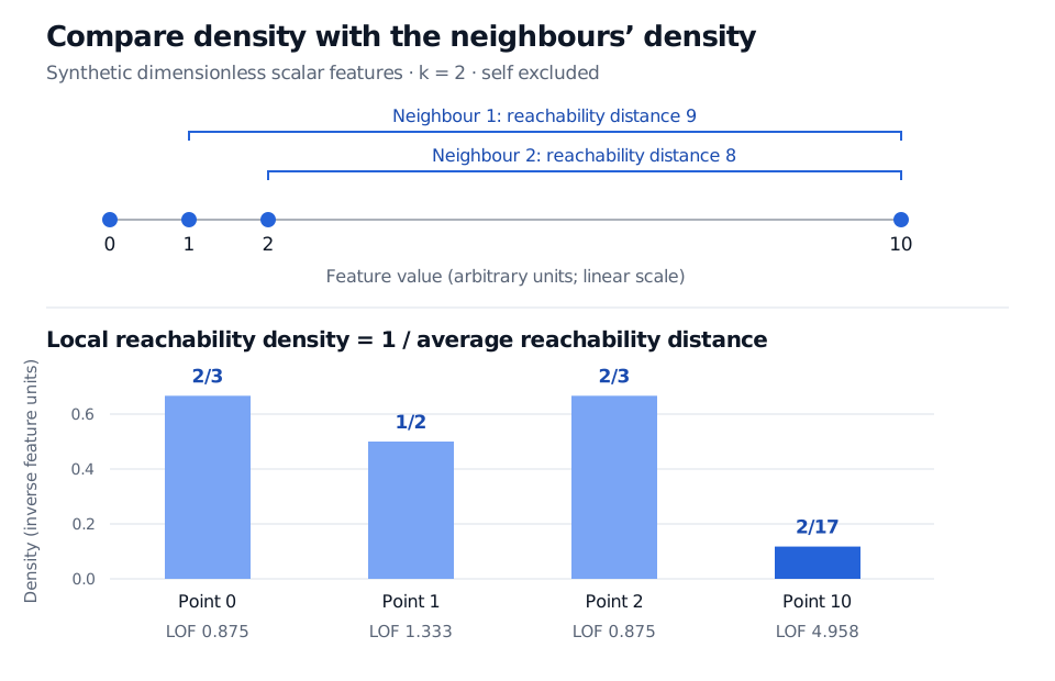
For point 10, the two reachability distances are max(1,9)=9 and max(2,8)=8. Their mean is 17/2, giving density 2/17. Its neighbours have mean density (1/2+2/3)/2=7/12, so
LOF2(10)=2/177/12=24119≈4.9583.
That means the neighbours’ average reachability density is about 4.96 times point 10’s density. It does not mean a 496% anomaly probability. Notice also that the middle point, 1, has score 4/3 despite sitting between 0 and 2: reachability smoothing changes its two distances from 1 to 2. “Above 1” alone is too crude a decision rule.
Synthetic scalar features 0, 1, 2 and 10 with k equal to 2 excluding self. Point 10 has neighbours 1 and 2, with reachability distances 9 and 8. Local reachability densities are 2/3, 1/2, 2/3 and 2/17; their LOF scores are approximately 0.875, 1.333, 0.875 and 4.958.
Original synthetic example. Point 10 is sparse relative to its two neighbours; the score compares densities rather than reporting a probability.
Scores, labels and future observations
The scikit-learn API reverses the sign for training scores: negative_outlier_factor_ is the negative of LOF, so more negative is more abnormal. A separate threshold produces binary labels. The contamination setting controls that threshold; it does not turn scores into probabilities or verify the prevalence of financial misconduct.
By default, fit_predict scores and labels the fitted sample. For later unseen observations, set novelty=True before fitting and use predict, score_samples or decision_function only on new data. In that mode, score_samples is an opposite LOF score; decision_function shifts it so negative values flag outliers. The official guide warns against applying these novelty methods to the training sample as a substitute for its stored scores. Verify neighbour and tie conventions before expecting software to reproduce a paper definition exactly.
What makes a financial peer comparison credible?
Features and distance determine who counts as a peer. A raw volume feature can dominate a spread feature through its units; irrelevant features can undermine local comparisons through the curse of dimensionality. Scaling all distances by the same positive constant leaves the density ratios unchanged, but rescaling only one feature can change the neighbourhoods.
The neighbour count sets the comparison scale. Small neighbourhoods can be unstable; large ones can blend different instrument types or market states. Inspect whether the unusual ranking survives reasonable choices. A compact group of problematic observations can also look ordinary relative to itself if its members supply one another’s neighbours.
For historical screening, build features, transformations and the reference sample using information available at the decision time. Later observations can alter earlier scores when included in a refit, creating look-ahead bias. A regime shift can produce many legitimate high scores. Investigate the original records and economic context before removing observations.
For a different density-based screening mechanism, the SelfMadeQuant anomaly-detection lesson develops Gaussian-mixture density thresholds (public preview; full lesson requires membership).