DBSCAN (Density-Based Spatial Clustering of Applications with Noise) groups observations through connected dense neighbourhoods and leaves sufficiently isolated observations labelled as noise. A quant can use it to explore peer groups in measured volatility or liquidity without specifying the number of groups in advance. A noise label means the observation did not meet this sample’s grouping rule; it does not establish a bad tick, fraud or a trading opportunity.
DBSCAN is an unsupervised learning method for clustering. Its groups can curve or stretch through feature space, because membership grows through local connections rather than around a single centre.
Core, border and noise
Choose a distance function, a neighbourhood radius (
eps) and a minimum count (min_samples). For observations , define the inclusive neighbourhoodFor ordinary, equally weighted observations:
- A core point has at least observations in its neighbourhood, including itself.
- A border point is not core, but lies within the radius of a core point.
- A noise point is neither core nor border.
Connect core points whose distance is at most , and take their connected components. Attach neighbouring border points to those components. Only core points propagate expansion: proximity to a border point alone does not pull another observation into the cluster. This is the mechanism behind the original algorithm, not a rule that every cluster member must have many neighbours.
Four observations, one cluster
Take the synthetic dimensionless scalar features . Use Euclidean distance, and , counting each observation itself. The scikit-learn DBSCAN API uses this self-counting convention.
| Observation | Neighbours within 0.15, including self | Count | Final role |
|---|---|---|---|
| 0 | 0 and 0.1 | 2 | Border |
| 0.1 | 0, 0.1 and 0.2 | 3 | Core |
| 0.2 | 0.1 and 0.2 | 2 | Border |
| 2 | 2 | 1 | Noise |
Only is core. Both and are close enough to that core point to join its cluster. The result is one cluster and noise point .
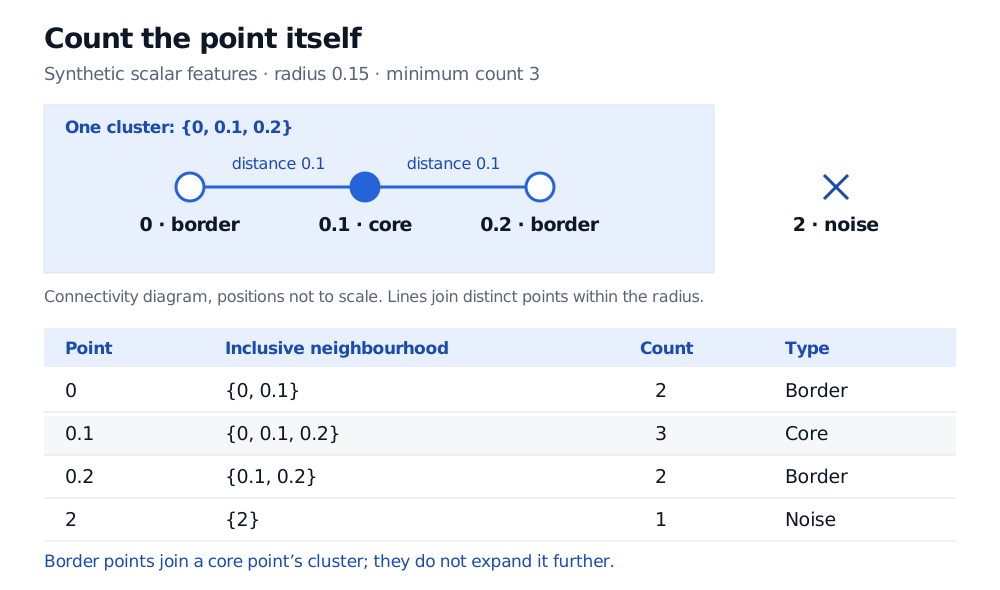
Original synthetic example. The neighbourhood table counts self; only the filled core point can expand the cluster.
Notice that the cluster’s endpoints are apart, exceeding the radius . The radius limits individual neighbourhood connections, not the total diameter of a cluster. Longer chains of core points can span much greater distances.
What changes the answer
Units change neighbourhoods. Multiply all four coordinates by ten but leave the radius at 0.15: every point becomes isolated and all four are noise. Increasing the radius to 1.5 restores the original grouping. With several features, rescaling just one changes relative distances, so standardising features is a modelling decision about what similarity should mean.
One density threshold can be too restrictive. A small radius may discard a genuine sparse group; increasing it may merge nearby dense groups. Inspect sensitivity to both parameters and the distance metric. HDBSCAN explores a hierarchy of density scales when a single threshold is unsuitable; it still requires interpretation and parameter choices.
Border membership can be ambiguous. A non-core point can lie within the radius of cores from two separate components. In scikit-learn, the component encountered first receives it. Permuting the data can therefore change that border assignment, while the grouping of core points remains unchanged. Numeric cluster IDs may also swap. The implementation discussion separates these two effects; “deterministic” does not mean every assignment is invariant to input order.
Unlike DBSCAN, k-means requires a chosen cluster count and assigns observations to centres. The k-Means Clustering lesson develops that method’s assignments and squared-distance objective (public preview; full lesson requires membership).
Reading the output in a quant workflow
Inspect groups and outliers in the original financial units. An isolated liquidity profile could reflect a valid unusual instrument, a changed market state or a measurement problem. DBSCAN alone cannot distinguish those explanations, and its noise label is not a calibrated anomaly or fraud probability.
If the grouping informs a historical decision, construct features, scaling and parameter choices using information available at that decision. Fitting on the complete history can introduce look-ahead bias even without outcome labels. Adding observations and refitting can change neighbourhood counts and cluster structure; state the update rule before treating the labels as a continuing economic classification.
Sources
- Martin Ester, Hans-Peter Kriegel, Jörg Sander and Xiaowei Xu, A Density-Based Algorithm for Discovering Clusters in Large Spatial Databases with Noise, KDD-96, pp. 226–231, §§3–4.1: neighbourhoods, core-based expansion and shared border points.
- Scikit-learn developers, DBSCAN API, parameters and attributes: self-counting
min_samples, radius meaning and fitted labels; stable documentation checked 1 November 2026. - Scikit-learn developers, Clustering: DBSCAN and HDBSCAN, §§2.3.7–2.3.8: parameter sensitivity, input-order effects and differing densities; stable documentation checked 1 November 2026.