L-moments and probability-weighted moments: Definition & Examples

L-moments describe a distribution through linear combinations of expected order statistics. Probability-weighted moments (PWMs) weight observations by their positions in the distribution; a particular PWM family generates the L-moments. For a quant comparing loss-severity distributions, they offer an alternative to cubing and taking fourth powers of losses when measuring shape.

Weight the probability, not the loss magnitude

For a continuous distribution with CDF

F

and quantile function

Q

, the general PWM family is

M_{p,r,s}=\mathbb{E}\!\left[X^p F(X)^r\{1-F(X)\}^s\right].

Use this general family only where the powers and expectation are defined. The family used here fixes $p=1$ and $s=0$ :

\beta_k=M_{1,k,0}=\mathbb{E}[X F(X)^k] =\int_0^1 Q(u)u^k\,du,\qquad k=0,1,\ldots.

Thus

\beta_0

is the mean. Higher

k

gives greater probability weight to the upper ranks, while

X

remains to the first power. This continuous-CDF identity should not be applied unchanged to a distribution with atoms. See Greenwood and colleagues' original definition.

The first four population L-moments are

\begin{aligned} \lambda_1&=\beta_0,\\ \lambda_2&=2\beta_1-\beta_0,\\ \lambda_3&=6\beta_2-6\beta_1+\beta_0,\\ \lambda_4&=20\beta_3-30\beta_2+12\beta_1-\beta_0. \end{aligned}

Equivalently, writing $X_{(j:r)}$ for rank $j$ in an independent sample of size $r$ ,

\lambda_r=\frac1r\sum_{k=0}^{r-1}(-1)^k \binom{r-1}{k}\mathbb{E}[X_{(r-k:r)}].

In particular,

\lambda_2=\tfrac12\mathbb{E}[|X-X'|]

for independent draws

X,X'

. It measures spread in the same units as

X

, unlike a variance. Hosking's paper develops this connection.

Four losses, with the normalization exposed

Take the fictional sorted loss sample $1,2,3,10$ , in USD millions. Assume independent observations from one continuous loss distribution when interpreting the sample quantities as population estimators.

For $n$ ordered observations, use the unbiased sample PWM estimator

b_k=\frac1n\sum_{i=1}^{n} \frac{\binom{i-1}{k}}{\binom{n-1}{k}}x_{(i)}, \qquad 0\le k\le n-1,

with $\binom{a}{k}=0$ when $a<k$ . Both the outer $1/n$ and the denominator $\binom{n-1}{k}$ matter.

For $n=4$ , the weights inside the sum for $b_1$ are $0,1/3,2/3,1$ . Hence

b_1=\frac14\left(0\cdot1+\frac13\cdot2+\frac23\cdot3+1\cdot10\right) =\frac{19}{6}.

The complete calculation is:

Quantity	Exact value	Meaning
$b_0$	$4$	Sample mean
$b_1$	$19/6$	First probability-weighted moment estimate
$b_2$	$11/4$	Second probability-weighted moment estimate
$b_3$	$5/2$	Third probability-weighted moment estimate
$\ell_1=b_0$	$4$	Sample L-location
$\ell_2=2b_1-b_0$	$7/3$	Sample L-scale
$\ell_3=6b_2-6b_1+b_0$	$3/2$	Third sample L-moment
$\ell_4=20b_3-30b_2+12b_1-b_0$	$3/2$	Fourth sample L-moment

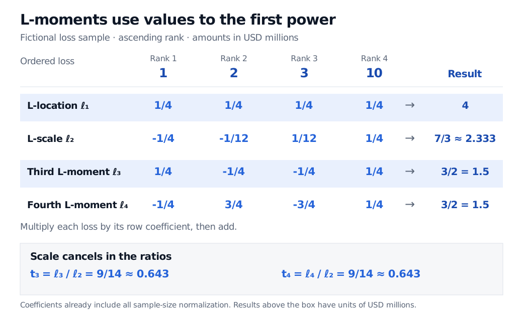
All eight entries have units of USD millions. The sample L-moments can also be calculated directly from the signed rank coefficients below.

Coefficient grid for fictional ordered losses of 1, 2, 3 and 10 USD millions. The rows produce sample L-moments of 4, 7/3, 3/2 and 3/2 USD millions. Sample L-skewness and L-kurtosis both equal 9/14, approximately 0.643.

Original fictional sample. Multiply each ordered loss by its row coefficient and add; the bottom panel divides the third and fourth L-moments by L-scale.

Using $F_n(x_{(i)})=i/n$ instead would give the plug-in estimate $\frac14\sum_i x_{(i)}(i/4)=27/8$ for $\beta_1$ , rather than $19/6$ . These are different finite-sample estimators. The combinatorial estimator corresponds to averaging order-statistic contrasts over all subsamples, as in Hosking's §3.1.

L-skewness and L-kurtosis are different scales

For a nonconstant population, define

\tau_3=\frac{\lambda_3}{\lambda_2},\qquad \tau_4=\frac{\lambda_4}{\lambda_2}.

Their sample versions give

t_3=\frac{\ell_3}{\ell_2}=\frac9{14}\approx0.643, \qquad t_4=\frac{\ell_4}{\ell_2}=\frac9{14}\approx0.643.

These dimensionless ratios are called L-skewness and L-kurtosis. Conventional skewness uses a third central moment divided by standard deviation cubed; conventional kurtosis uses a fourth central moment divided by variance squared. Their values are not interchangeable with

\tau_3

and

\tau_4

. In particular, subtracting three from L-kurtosis does not turn it into conventional excess kurtosis.

A software detail can otherwise create a misleading comparison: Hosking's R package lmom returns

\ell_1,\ell_2,t_3,t_4

by default from samlmu, while ratios=FALSE returns

\ell_1,\ell_2,\ell_3,\ell_4

. Check the official function documentation before treating its third and fourth outputs as amounts.

What the extra stability buys—and what it cannot

The untrimmed population L-moments exist when $\mathbb{E}[|X|]<\infty$ , even if variance or higher conventional moments fail to exist. Existence alone does not give finite estimator variance or justify a normal confidence interval. Unbiased $b_k$ and $\ell_r$ also do not make their ratios unbiased.

Less sensitivity to extremes is useful for distribution fitting, but it is not outlier immunity. In this very sample, replace the largest loss by $M\ge3$ . Then

\ell_1=\frac{M+6}{4},\qquad \ell_2=\frac{3M-2}{12}.

Both grow without bound. A data error can still dominate untrimmed L-location and L-scale. If all observations are equal,

\ell_2=0

and the shape ratios are undefined. Trimmed L-moments are a separate family, explicitly distinguished in the package documentation.

For fitting, the method of L-moments matches sample L-moments to those of a chosen distribution, paralleling the ordinary method of moments. It still requires a defensible distribution family and a sampling design; four illustrative losses cannot validate an extreme loss forecast.

For the underlying rank notation and sampling distributions, Order Statistics and Sample Quantiles develops order-statistic densities and contrasts the behaviour of means and medians. A public preview is available; the full lesson requires membership.

Sources

Greenwood, Landwehr, Matalas and Wallis (1979), Probability weighted moments: Definition and relation to parameters of several distributions expressable in inverse form, definition (3) and the order-statistic connection (5).
Hosking (1990), L-moments: Analysis and Estimation of Distributions Using Linear Combinations of Order Statistics, §§2.1–2.4 and 3.1–3.4.
Hosking, lmom package reference manual, package overview, trimmed L-moments, and samlmu arguments and return values.

Weight the probability, not the loss magnitude

Four losses, with the normalization exposed

L-skewness and L-kurtosis are different scales

What the extra stability buys—and what it cannot

Sources

Related terms

Cumulative distribution function

Method of moments

Quantile function