Kernel principal component analysis (kernel PCA) finds principal components after a nonlinear feature transformation, using kernel evaluations instead of explicitly constructing the transformed features. For a quant compressing market indicators, it can capture variation in nonlinear combinations of those indicators. The resulting components maximise variance in the chosen feature space; they need not be tradable portfolios or the directions most useful for predicting returns.
The kernel trick supplies an inner product . Kernel PCA applies ordinary PCA to the centered versions of . A linear kernel recovers ordinary centered PCA. The nonlinear feature-space interpretation is the defining construction in Schölkopf, Smola and Müller's original paper.
Center the features, then find their directions
For training observations, form the Gram matrix . Use a real symmetric positive semidefinite kernel. Let be the length- vector of ones and set
This subtracts the training mean in feature space, . Centering the input coordinates before applying a nonlinear map generally does not do that job. Appendix B of the original paper derives both training and test centering.
For a positive eigenvalue of , choose a Euclidean unit eigenvector . The corresponding unit direction in feature space is
The training component scores are therefore
An eigenvector alone is not the score vector: its scale must be restored. Zero eigenvalues supply no nonzero feature direction and cannot be used in this division. Reversing an eigenvector's sign reverses its scores without changing the component subspace.
Three inputs make the normalization visible
Take fictional unitless inputs and the homogeneous quadratic kernel
The input mean is already zero, but the feature values are , with mean . Their centered values form
This rank-one matrix has eigenvalues . Choose
Then : the scores are , up to a common sign. They are not these values divided by .
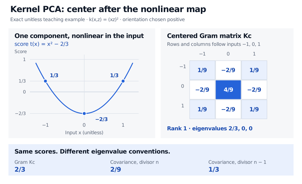
Original deterministic example. The curve shows the fitted score map, not a financial forecast. Equal scores at opposite inputs reveal the sign information discarded by this kernel.
The eigenvalue convention explains the tempting extra factor. Here belongs to the Gram matrix. The feature covariance with divisor has nonzero eigenvalue ; with divisor , it is . The scores stay the same. Software output called “eigenvalues” must be interpreted according to the matrix it diagonalizes; scikit-learn's KernelPCA documentation explicitly identifies the centered kernel matrix.
For a fixed kernel and training set, measures the fraction of centered feature-space variance retained. In this example, one component retains all such variance, yet and have become indistinguishable. Retained feature variance does not establish retained information about the original input, economic risk or a prediction target.
A new observation keeps the training origin
For a new input , first evaluate . Center each entry using training quantities:
Its score on component is
For in the example, the raw kernel vector is , the centered vector is , and the score is . Direct feature centering independently gives . Re-estimating the origin from the test batch would change the fitted transformation. The official KernelCenterer documentation describes retaining the fitted training-column and overall kernel means.
What the representation does not promise
A kernel PCA score does not automatically have an inverse in input space. Here the score corresponds to both and . More generally, a projected feature vector may have no exact pre-image at all. An approximate reconstruction requires an additional method; scikit-learn's optional inverse transform learns a pre-image through kernel ridge regression.
The kernel and its input scales also determine which variation looks large. A visually separated embedding is not evidence of future predictive performance. For forecasting, fit scaling, kernel centering and component directions inside each training window; choose kernel settings and component count using a time-respecting validation design, and transform later observations with that fitted mapping. The training-only transformation rule follows the official guidance on preprocessing leakage. Full dense kernel storage also grows as , so avoiding explicit features does not eliminate sample-size costs.
To build the linear foundation, the SelfMadeQuant lesson Principal Component Analysis and the SVD View develops the maximum-variance direction. The Kernel Trick develops feature maps and Gram matrices. Both offer public previews; full lessons require membership.
Sources
- Schölkopf, Smola and Müller (1998), Nonlinear Component Analysis as a Kernel Eigenvalue Problem: §2, §6.3.5 and Appendix B for feature-space PCA, normalization, computational limits and centering.
- scikit-learn, KernelPCA API: centered-kernel eigenvalues and the separately learned approximate inverse.
- scikit-learn, KernelCenterer API: fitted training means for feature-space centering.
- scikit-learn, Common pitfalls, §§12.1–12.2.1: consistent preprocessing and training-only fitting.