The phrase is sometimes used informally for a list of available data. The mathematical object records the distinctions those data allow you to make. Two differently formatted datasets can therefore represent the same information set.
A signal reveals the regime, not the loss
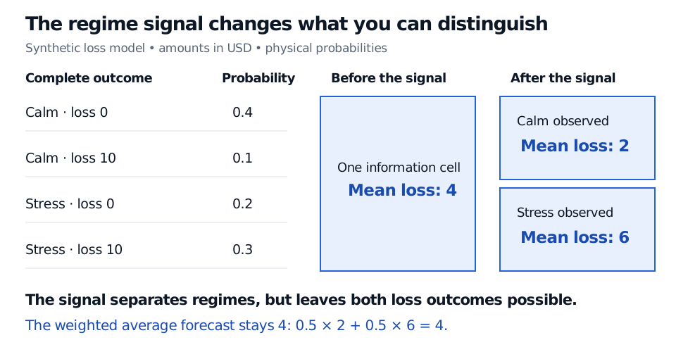
Consider a synthetic one-period position whose loss is either USD 0 or USD 10. A regime signal is released before the loss is observed. The model assigns these joint probabilities:
| Regime | Loss (USD) | Probability |
|---|---|---|
| Calm | 0 | 0.4 |
| Calm | 10 | 0.1 |
| Stress | 0 | 0.2 |
| Stress | 10 | 0.3 |
Before the signal, suppose the observer has no information distinguishing these four outcomes. Their information set is the trivial sigma-algebra , and the expected loss is
After the signal, the observer can answer “Is the regime calm?” but still cannot answer “Will the position lose USD 10?” The information set is now , with exactly four events: the empty event, calm, stress and the entire sample space. Observing calm leaves two possible outcomes; observing stress also leaves two.
This is a random variable before the signal arrives, taking the value USD 2 or USD 6 depending on what is revealed. It is a forecast of loss, not the realised loss or a derivative price. No discounting or risk-neutral valuation is being assumed.
More information means more distinguishable events
The relation means that every event distinguishable with is also distinguishable with . In the finite example, the new information splits a single cell into calm and stress cells. The number of data columns is not the criterion: a copied column adds no information, while a timely new signal can split previously indistinguishable outcomes.
A loss forecast using only the regime must assign the same value to both calm outcomes and the same value to both stress outcomes. This is what -measurability means here. A forecast equal to the eventual realised loss would fail that test: it distinguishes outcomes the signal has not separated.
More information does not guarantee a lower loss forecast. Stress raises it from USD 4 to USD 6. Averaging across the possible signals recovers the original expectation, an instance of the tower property:
Nor does observing the signal itself lower the position's realised loss. A better-informed decision may change exposure, but profitability and risk depend on the decision, prices, costs and the model's accuracy.
Whose information, available when?
Sources
- Steven E. Shreve, Stochastic Calculus and Finance, CMU lecture notes prepared by Prasad Chalasani and Somesh Jha, 25 July 1997, §2.2 (information determined by observations and generated sigma-algebras), §§2.3.3–2.3.4 (conditioning on a sigma-algebra and its properties). The regime-and-loss model is original.
- Samuel Drapeau, Stochastics: Discrete Time Processes, “Stochastic Process, Filtration, Adaptiveness”: information represented by nested sigma-algebras and measurability relative to current information.