A market-making control model combining tick-valued spread states, priority-dependent limit fills and immediate market-order impulses to manage inventory.
Guilbaud–Pham market-making model
The Guilbaud–Pham market-making model is a stochastic-control model in which a small market maker chooses limit-order prices and sizes while retaining the option to trade immediately with market orders. Its practical question is whether to wait for a better execution price, improve a quote to increase its execution rate, or pay the spread to change inventory now.
The distinctive combination is a spread that switches between tick-sized states, execution rates that depend on quote priority, and a joint decision over passive quotes and immediate trades. This extends the basic economics of market making into a finite-horizon control problem. The reference here is Guilbaud and Pham's 2011 preprint, §§2–3.
Two ways to change the position
Let Xt be cash, Yt inventory in shares, Pt the midpoint and St the full bid-ask spread. The outside best bid and ask are Pt−St/2 and Pt+St/2.
Limit orders are regular controls. The maker continuously chooses a buy size Ltb, a sell size Lta, and whether each quote joins the corresponding best price or improves it by one tick δ. Sizes are bounded and may be zero. Improving the bid means paying one tick more; improving the ask means receiving one tick less. In exchange, the model assigns the improved quote a higher execution intensity. At a one-tick spread, improvement would reach the opposite quote and is treated as a market order instead.
The limit order fills remain uncertain. With Nb counting executions of the maker's bid and Na executions of its ask, the accounting is
Here πb and πa are the maker's execution prices, with rebates incorporated if specified. A filled bid spends cash and adds shares; a filled ask receives cash and removes shares. The paper models these executions with Cox counting processes whose intensities depend on the chosen quote and prevailing spread. An intensity is an arrival rate per unit time, not a fill probability over an unspecified horizon. §2.2, equations (2.2)–(2.3).
Market orders are impulse controls. At chosen stopping times, the maker submits a signed quantity e: positive to buy, negative to sell. The state jumps to
(X,Y)⟼(X−c(e,P,S),Y+e),c(e,p,s)=ep+∣e∣s/2+ε.
For an actual nonzero trade, ε is a fixed fee in this specification. Buying pays the ask; selling receives the bid, less the fee. The small-agent assumption makes execution immediate at that price for the admissible size. It excludes walking through multiple book levels. §2.2, equations (2.4)–(2.5).
A spread state is different from a quote choice
The spread takes finitely many values δ,2δ,…,mδ. A discrete Markov chain determines its successive states and an independent Poisson clock determines when it changes. In calendar time this gives a continuous-time Markov chain, possibly with time-dependent jump rates. The paper assumes the midpoint and spread processes are independent and exogenous.
The maker's improved quote changes its own execution opportunity; it does not endogenously reset the model's outside spread. Queue priority is represented through execution rates rather than an explicit simulation of every order ahead. These distinctions matter when adapting the model to data with latency or rapidly changing competition. §§2.1–2.2.
A one-share ledger, before calling anything optimal
Suppose the maker already owns one share, marked at USD 100, with an outside bid of 99.98, ask of 100.02 and tick of 0.01 dollars per share. Compare three selling actions over one stipulated decision window. Freeze prices, omit fees and rebates, allow at most one fill, and stipulate fill probabilities of 60% at the ask and 90% after improving the ask. These are fictional inputs, not calibrated estimates or probabilities derived from the paper's intensities.
Selling action
Cash received if filled (USD)
Shares left if unfilled
Expected gain marked at unchanged midpoint (USD)
Post at ask
100.02
1
0.60(100.02−100)=+0.012
Improve ask one tick
100.01
1
0.90(100.01−100)=+0.009
Sell at bid now
99.98
No unfilled branch
99.98−100=−0.020
All gains are relative to the initial one-share midpoint value, not profits relative to the share's purchase cost. The expected remaining inventories are 0.4, 0.1 and 0 shares, respectively. The market sale gives up two cents of marked value and removes the position immediately. A passive order can leave the entire share exposed to inventory risk.
Now change just the end-of-window convention: sell every unfilled share at the unchanged bid. The first action's expected completed gain becomes
0.60(0.02)+0.40(−0.02)=0.004 USD.
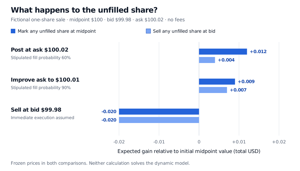
The improved ask gives 0.90(0.01)+0.10(−0.02)=0.007 USD. The immediate market sale still gives −0.020 USD. Completing the no-fill branch reverses the comparison between the two passive alternatives, even with frozen prices and no risk penalty.
Fictional one-share sale: expected gains at an unchanged midpoint are USD 0.012 at the ask, 0.009 at the improved ask and minus 0.020 at market. Selling unfilled shares at the unchanged bid changes them to 0.004, 0.007 and minus 0.020.
Original fictional action ledger. Dark bars mark remaining inventory at the midpoint; light bars sell it at the bid. The comparison changes because unfilled inventory has a liquidation cost.
Neither comparison solves the Guilbaud–Pham model. Both omit price changes, future quote revisions, repeated execution opportunities, fees and a full risk objective. A higher expected marked gain alone cannot identify the optimal policy. Nor do the stipulated fill probabilities describe adverse selection: that requires considering price behaviour conditional on execution.
What the dynamic optimisation adds
The paper's value function maximises expected utility of terminal liquidation wealth, less a running inventory penalty:
Here L is cash after closing the remaining position with a market order, including spread and applicable fees. The paper starts from terminal flat inventory and represents liquidation in the terminal payoff. Its examples include linear reward U(x)=x with g(y)=y2 and a positive penalty weight, and exponential utility with no separate running penalty. A quadratic inventory penalty is not automatically the variance of terminal P&L. §3.1, equations (3.1)–(3.3).
Dynamic programming gives a quasi-variational inequality:
min{−∂tv−Q,LsupAQ,Lv+γg(y),v−Mv}=0.
AQ,L describes midpoint and spread evolution plus limit fills under admissible quotes and sizes. Mv is the best continuation value after an admissible market-order impulse, with its cash cost deducted. The first branch governs continuing with limit controls; the second allows immediate intervention. At the terminal date, v=U(L). The optimisation compares future state values, not simply today's spread revenue. §3.2, equations (3.4)–(3.6).
Finally, the rates must be estimated. Section 2.3 separates spread-transition estimation from execution-rate estimation: executions in a quote/spread state are divided by time exposed in that state. The paper also constructs execution proxies when actual strategy fills are unavailable. Such proxies do not establish that an untraded historical quote would really have filled. The value of the control solution remains conditional on the execution model and its assumptions.
Sources
Guilbaud, F. and Pham, H. (2011), Optimal high frequency trading with limit and market orders, arXiv:1106.5040v1, 24 June 2011. Sections 2.1–2.3 specify spread states, controls, accounting and estimation; §§3.1–3.3 formulate the objective, QVI and special-case reductions. The numerical ledger above is an original fictional illustration, not a reproduced empirical result.