Compare algorithm ranks across independent datasets, calculate Friedman and Nemenyi results, and distinguish approximate significance from economic value.
Friedman test and Nemenyi post-hoc comparison
The Friedman test compares three or more methods using their ranks within the same independent dataset blocks. Nemenyi post-hoc comparison then tests all pairs of average ranks. A quant can use this combination to compare forecasting algorithms across separate prediction problems without treating their raw loss scales as interchangeable.
The omnibus hypothesis test asks whether the methods have the same expected rank under the null of exchangeable method labels within blocks. Rejection does not identify the differing pairs; that is the post-hoc question. Demšar (2006, §3.2.2) explains this design for algorithm comparisons.
Five datasets, three algorithms
This is a stipulated example, not measured financial performance. Algorithms A, B and C are evaluated on five independent datasets using one predeclared metric; rank 1 is best and there are no ties.
Dataset block
A
B
C
1
1
2
3
2
1
2
3
3
1
3
2
4
2
1
3
5
1
2
3
Average rank
1.2
2.0
2.8
Let N be the number of datasets, k the number of algorithms, and Rj algorithm j's average rank. For untied ranks, the Friedman statistic is
Q=k(k+1)12Nj=1∑kRj2−3N(k+1).
Here N=5, k=3, so
Q=5(1.22+22+2.82)−60=6.4.
Using the asymptotic chi-squared distribution with k−1=2 degrees of freedom gives a p-value of 0.04076. This crosses a predeclared 5% omnibus threshold under that approximation.
Five blocks are a small sample. This is not an exact finite-sample p-value: SciPy's Friedman documentation explicitly cautions about small samples. An exact or permutation reference requires a valid exchangeability design; the chi-squared calculation alone does not establish it.
Which pair clears the critical difference?
For the conventional Nemenyi all-pairs reference,
CD=qα6Nk(k+1),qα=2q1−α;k,∞range.
The second expression specifies the convention: divide the studentized-range quantile by 2. At α=0.05 and k=3, qα≈2.34370, giving CD≈1.48229. The SciPy studentized-range distribution supplies the quantile; Demšar's Table 5 uses the divided convention.
Pair
Absolute average-rank gap
Exceeds CD?
A–B
0.8
No
B–C
0.8
No
A–C
1.6
Yes
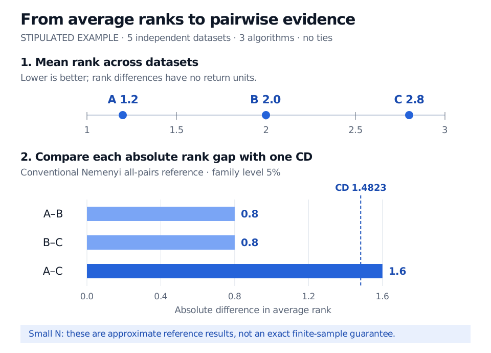
Only A–C is separated by this conventional approximate procedure. A–B and B–C non-rejection does not establish equivalence, or make A–C non-rejection follow by transitivity.
Stipulated five-independent-dataset example: average ranks A 1.2, B 2.0 and C 2.8. A–B and B–C gaps are 0.8; the A–C gap of 1.6 alone exceeds the approximate 5% Nemenyi critical difference of 1.4823.
Original calculation from the stipulated ranks. The common CD adjusts for the all-pairs family; small-sample approximation remains a limitation.
Choose the comparison before looking at the ranks
Nemenyi targets all pairs and family-wise error. A predesignated control-versus-challengers question has a different comparison family. Do not select that control after seeing the winner. Demšar (§3.2.2) distinguishes these designs.
The dataset is the replication unit. Cross-validation folds from one dataset are not independent dataset blocks; correlated assets do not become independent simply because each has its own ticker. Demšar (§3 and §3.2.3) separates dataset replication from resampling. The membership lesson Finance-aware validation develops overlapping-label and time-dependence issues; its public page is a preview.
For ties, assign average ranks and use a tie-corrected Friedman calculation. SciPy documents that correction; the untied formula and CD illustration above should not be copied unchanged into a heavily tied experiment.
Ranks discard magnitude. A tiny loss improvement and a large one can generate the same ordering. Alongside the rank analysis, report raw out-of-sample metrics, uncertainty, trading costs and exposure constraints. Neither the lowest average rank nor a rejected pairwise null establishes a profitable strategy.