The 52-week high effect ranks stocks by proximity to a recent peak. Define the price window, distinguish momentum, and separate historical evidence from trading profits.
52-week high effect
The 52-week high effect is the historical finding that stocks trading nearer their own previous year's high tend to earn higher subsequent returns than stocks trading farther below it. For a quant researcher, the useful distinction is between proximity to a peak and momentum measured by past returns: they can rank stocks differently. George and Hwang's 2004 study found that the price-to-high measure contained predictive information beyond past individual-stock and industry returns. That is an empirical result from historical data, not a rule that a stock near its high must keep rising. George and Hwang, 2004.
Build the ranking before discussing the trade
One explicit daily version uses a positive split-adjusted closing-price series, with all prices expressed in consistent share units:
Hi,t=j=0,…,251maxPi,t−j,Si,t=Hi,tPi,t.
Here Pi,t is stock i's closing price on trading day t, Hi,t is the highest close among the 252 observations ending today, and Si,t is its proximity score. A larger score means nearer the high. With today's close included, 0<Si,t≤1. A score of 1 means the current close equals the window's maximum; it says nothing about the next return.
The window and price field are choices, not details to leave to a vendor default. A trailing 12-calendar-month window need not contain 252 sessions. The maximum daily close differs from the maximum intraday high. George, Hwang and Li's later study explicitly uses the highest daily closing price, adjusted for splits and stock dividends, over the past 12 months; our 252-observation version is an illustration rather than a replication of their calendar rule. Excluding today from the maximum creates another version whose ratio can exceed 1. George, Hwang and Li, §3.
Consider two fictional stocks with complete 252-observation histories:
Stock
Current adjusted close
Maximum adjusted close
Proximity score
A
$90
$100
0.90
B
$50
$100
0.50
A ranks above B. These observations alone do not establish a profitable trade. Suppose a subsequent, stipulated one-month holding period produces total returns of +2% for A and +1% for B, measured from executable entries to exits. A position initially long $100 of A and short $100 of B earns $2 minus $1, or $1 before costs. The long-minus-short return spread is 1 percentage point; it is not automatically a 1% return on the trader's equity, which depends on capital, margin and financing. One invented outcome does not test the anomaly.
Same past return, different signal
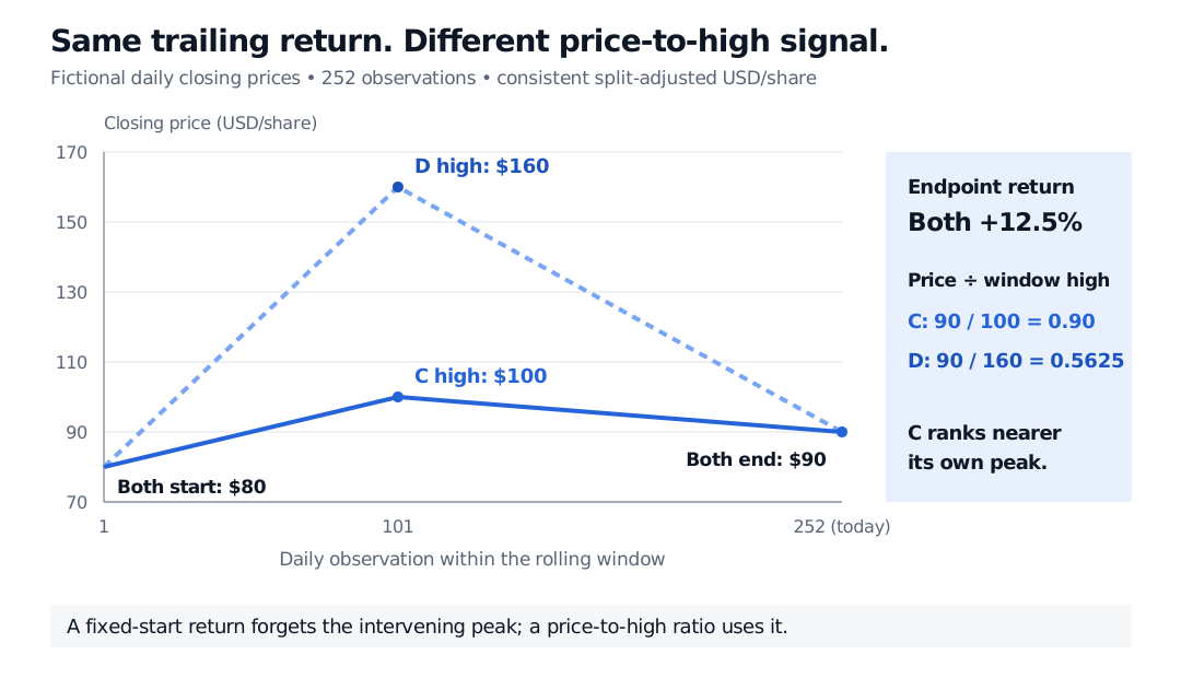
A return compares the endpoint with a selected starting price. Proximity also uses the intervening peak. In the fictional paths below, C and D both rise from $80 to $90 over the window, a 12.5% price return. C reaches a maximum of $100; D reaches $160. Their proximity scores are therefore 0.90 and 0.5625. C ranks nearer its high despite having exactly the same endpoint return as D.
Fictional 252-observation closing-price paths C and D both start at $80 and end at $90, a 12.5% price return. C peaks at $100 and has proximity 0.90; D peaks at $160 and has proximity 0.5625.
Fictional daily paths with identical start and end prices. The intervening maximum changes the price-to-high ranking without changing the trailing endpoint return.
A reference point is an explanation to test
George and Hwang propose anchoring as an interpretation: investors may use the salient annual high as a reference point and underreact to information that warrants a price beyond it. Their evidence is about subsequent portfolio returns, not a guarantee that touching the high triggers a breakout. Original manuscript, introduction and §I.
A behavioural interpretation is not the only possibility. George, Hwang and Li's 2018 research connects price-to-high to future profitability and investment growth and finds that an investment-based q-factor model helps capture the return pattern. Its findings do not establish that investors never misprice stocks. The relevant research question is whether proximity adds information after the chosen risk controls, related signals and implementation costs—not whether the ratio can be calculated. George, Hwang and Li.
Small data choices can change the conclusion
Keep share units consistent. After a two-for-one split, a pre-split $120 high corresponds to $60 in current share units. A $54 close is then 0.90 of that high; dividing it by the unadjusted $120 invents a 0.45 score. Document cash-dividend treatment too: a split-adjusted price high and a total-return-series high answer different questions. Vendor adjustment policies differ, including when adjustments are applied. QuantRocket's data guide describes these distinctions.
Respect information arrival. Today's completed closing bar is unavailable before the close. A signal calculated from it needs a later feasible execution, with the actual delay and fill price reflected in returns. Assuming entry at that same close can introduce look-ahead bias. Declare any skipped month and the holding horizon; changing either changes the experiment.
Keep the historical opportunity set. Use eligibility and index membership as they were at each formation date, retain delisted securities and handle terminal returns. Screening past data using only today's survivors introduces survivorship bias. State how new listings, missing observations and tied scores are treated.
Separate a return spread from usable profits. Rebalancing incurs transaction costs; a short leg also needs borrow availability, borrow fees and distribution payments. Test later periods and other eligible universes, and account for the many windows and portfolio rules tried. A historical gross ranking effect can weaken or disappear after these choices.
For a worked treatment of split units, distribution accounting and historical membership, see Corporate Actions and Survivorship (public preview; full lesson requires membership).
When the old high leaves the window
A stock closes at $96. Its 252-close window has a $120 maximum in the oldest observation, with all other closes at or below $100 and at least one equal to $100. Tomorrow the $120 observation drops out, the $100 observation remains, and the stock again closes at $96. Has the stock earned a positive return because its proximity score rose?
Answer. No. The score rises from 96/120=0.80 to 96/100=0.96, while the close-to-close price return is 96/96−1=0. A rolling reference point can change even when the stock price does not. An increase in proximity is therefore not, by itself, evidence of new buying pressure or a positive realised return.
QuantRocket, Usage Guide: US Stock, split and dividend adjustments, delisted stocks, and comparison of history databases with point-in-time bundle adjustments; accessed 30 October 2026.