EVaR minimises an exponential bound on loss risk. Derive its normal-loss formula, compare it with VaR and ES, and recognise its sensitivity to tail assumptions.
Entropic value at risk
Entropic value at risk (EVaR) is a loss risk measure obtained by minimising an exponential probability bound over its tuning parameter. It gives a conservative alternative to value at risk and expected shortfall, with a form useful in portfolio optimisation. Its conservatism is relative to the specified loss distribution: a larger number does not establish that the model captures real crashes.
From a probability bound to a monetary threshold
Let L be loss over a fixed horizon, with positive values denoting losses and negative values gains. Write α for confidence and p=1−α for the upper-tail probability. Thus 99% confidence means p=0.01; confusing these conventions reverses the intended tail emphasis.
The moment-generating function is ML(θ)=EeθL]. For any θ>0 where this expectation is finite, the [Chernoff bound gives
P(L≥x)≤e−θxML(θ).
Setting the right side equal to p produces a loss threshold
bp(θ)=θlogML(θ)−logp.
EVaR takes the smallest threshold available from this family:
EVaRα(L)=θ>0infθlogE[eθL]−log(1−α).
Infinite exponential moments contribute an infinite objective. The infimum notation matters: a finite positive optimiser need not exist. For a certain loss L=c, the objective is c−log(p)/θ and approaches c only as θ→∞.
If L is in USD, θ is in inverse USD, making the exponent dimensionless and EVaR a USD amount. Under the usual finite-domain conditions, the same-confidence ordering is VaRα≤ESα≤EVaRα. EVaR is an upper bound, not the average of the worst p fraction of losses; that average is ES. Ahmadi-Javid's original paper introduces this construction.
A normal loss where the minimisation is explicit
Suppose a fictional one-day monetary loss follows a normal distribution with mean USD 1 and standard deviation USD 2. These are stipulated loss-model parameters, not estimates from market observations. In USD numerical units, L∼N(1,22).
For a general normal loss with mean μ and standard deviation σ>0,
logML(θ)=μθ+2σ2θ2,bp(θ)=μ+2σ2θ−θlogp.
Differentiating gives bp′(θ)=σ2/2+log(p)/θ2. Its zero yields
θ∗=σ−2logp,EVaRα(L)=μ+σ−2logp.
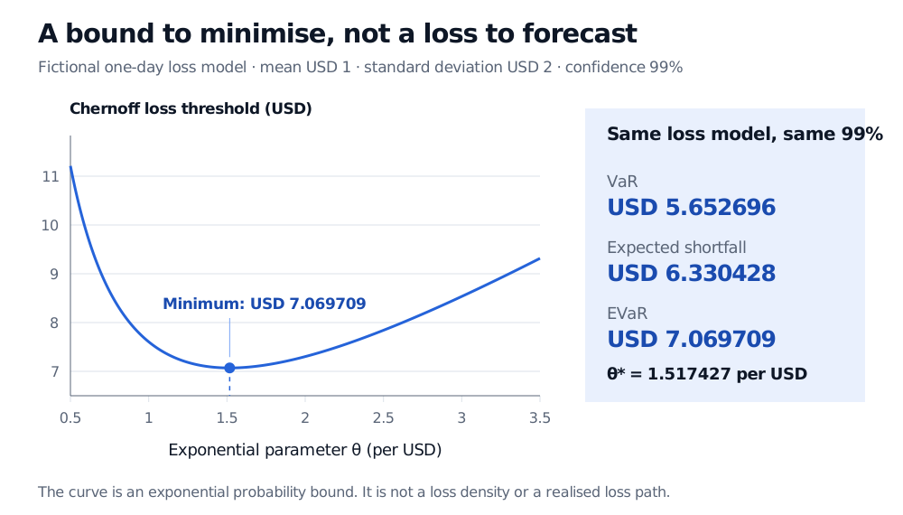
At 99% confidence, θ∗≈1.517427 per USD and EVaR is USD 7.069709. Choosing θ=1 per USD would instead give a looser threshold of USD 7.605170.
For comparison, put z=Φ−1(0.99), where Φ and ϕ are the standard normal CDF and density. VaR is μ+σz and ES is μ+σϕ(z)/0.01.
Same one-day normal loss model
USD
Meaning
99% VaR
5.652696
Exact model quantile
99% ES
6.330428
Model average of the worst 1%
99% EVaR
7.069709
Optimised exponential-bound threshold
Fictional one-day normal USD loss with mean 1 and standard deviation 2. At 99% confidence the exponential bound is minimised at theta 1.517427 per USD, giving EVaR USD 7.069709. VaR is USD 5.652696 and expected shortfall is USD 6.330428.
Original fictional normal-loss example. The curve plots the Chernoff loss threshold against its exponential parameter; its minimum defines EVaR. All three risk measures use the same one-day distribution and 99% confidence.
The normal model's actual probability of exceeding USD 7.069709 is about 0.120326%, below the 1% Chernoff bound. The gap is the price of using this bound. EVaR is neither an exact 99th percentile nor a maximum possible loss; this normal distribution has no finite upper endpoint.
For the standardisation behind that probability check, the Normal Distribution lesson develops normal tail calculations. Its public page is a preview; the full lesson requires a free signed-in account.
What the exponential emphasis changes
Large positive losses receive exponentially increasing weight inside ML(θ). A finite sample can therefore make EVaR computable while leaving substantial uncertainty about the population tail. A nondegenerate lognormal positive loss, for example, has finite ordinary moments but no finite positive exponential moment, so its population EVaR is infinite; the Virtual Laboratories notes, “Moments,” give this contrast. Every finite empirical sample of that distribution has finite EVaR. A finite software result does not settle the existence question for the underlying model.
EVaR is a coherent risk measure on its appropriate domain. It respects loss ordering and certain-loss shifts, scales proportionally with nonnegative exposure, and is subadditive. Subadditivity compares combined risk with the sum of standalone risks; it does not say that adding a position always reduces risk. These properties support portfolio aggregation, but they do not insert missing liquidity costs or dependence scenarios into L.
The name “entropic” also has a precise interpretation. For bounded losses, EVaR equals the largest expected loss obtained by reweighting the reference probabilities within a relative-entropy budget of −logp. Delbaen's analysis, §1, states this dual representation using the opposite, utility sign convention. The budget limits probability distortion; it does not protect against every imaginable loss model or create outcomes absent from the reference model.
Finally, the entropic risk measure at a fixed parameter is ρθ(L)=logE[eθL]/θ. EVaR adds −logp/θ and then optimises over θ. A chosen risk-aversion parameter and a chosen confidence level are different inputs. Neither calculation by itself establishes a regulatory capital requirement.
Sources
Amir Ahmadi-Javid, Entropic Value-at-Risk: A New Coherent Risk Measure, Journal of Optimization Theory and Applications 155, 1105–1123 (2012; online December 2011). The checked publisher abstract establishes the original construction and its relation to VaR, CVaR and entropy; full subscription text was not used.
Amir Ahmadi-Javid and Malihe Fallah-Tafti, Portfolio Optimization with Entropic Value-at-Risk, author manuscript, §2, equation (2-1), normal comparison and Remark 1; §3.2. These supply the defining formula, domain discussion and sample-based optimisation setting. The USD scenario, calculations and figure here are original.
Virtual Laboratories, The Lognormal Distribution, “Moments,” exercises 8–10, hosted by Universidad Nacional de Mar del Plata. This gives finite ordinary moments alongside divergence of every positive exponential moment.