A model that assigns low energy to compatible states; exponentiation and a finite partition function turn its scores into probabilities.
Energy-based model
An energy-based model (EBM) assigns a scalar energy to a possible configuration, with lower energy indicating greater compatibility. A probabilistic EBM converts these scores into a probability distribution by exponentiating their negatives and normalizing. For a quant using the model for scenario generation or unusual-observation detection, this distinction matters: an energy score alone is neither a scenario probability nor a tail-risk estimate.
The broader energy-based framework also includes models used only to choose a low-energy answer, without defining probabilities. LeCun and Huang make this distinction explicitly. Here the focus is the probabilistic construction.
Here θ contains the model parameters and T>0 is temperature. The energyEθ(x) is a score; exp(−Eθ(x)/T) is an unnormalized positive weight; the partition functionZθ,T makes those weights sum to one. It is constant across states for a fixed model and temperature, but generally changes when the parameters change.
Consider three fictional states with dimensionless energies and T=1:
State
Energy
Unnormalized weight
Probability
A
0
1
4/7
B
ln2
1/2
2/7
C
ln4
1/4
1/7
The weights total Z=7/4. Dividing each weight by 7/4 gives the last column. Equivalently, the odds are 4:2:1, so seven equal units of mass are allocated as four, two and one. Choosing the minimum-energy state always selects A; sampling from this distribution can also select B or C.
These numbers are an arithmetic example, not probabilities estimated from market data. Naming A a “normal regime” and C a “crash regime” would not make the model a validated crash forecaster.
Only energy differences determine the law
For two states in the same model,
pθ,T(b)pθ,T(a)=exp(−TEθ(a)−Eθ(b)).
Adding the same constant c to every energy multiplies all weights and the partition function by exp(−c/T). The probabilities stay unchanged. Adding five to the example's energies therefore preserves 4/7, 2/7 and 1/7, even though the partition function becomes much smaller. Negative energies are allowed; the energy zero is arbitrary.
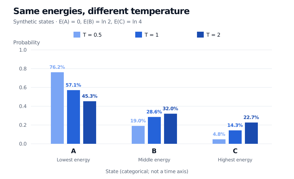
Temperature changes the relative odds. Under the convention used here, raising T flattens the distribution and lowering it concentrates mass on the lowest-energy states. Some sources write exp(−βE) instead, where inverse temperatureβ=1/T; others absorb temperature into the energy and simply write exp(−E). Compare conventions before comparing numerical scores.
Three fictional states with energies zero, ln 2 and ln 4. At T=1 their probabilities are 57.1%, 28.6% and 14.3%. At T=0.5 they are 76.2%, 19.0% and 4.8%; at T=2 they are 45.3%, 32.0% and 22.7%.
Figure: Holding energies fixed, lower temperature concentrates probability on A and higher temperature flattens the three-state law.
A common energy shift changes nothing, whereas multiplying all energies at a fixed temperature generally changes the distribution. Multiplying both energies and temperature by the same positive factor preserves it.
A continuous energy need not define a density
For a continuous state x∈Rd, replace the sum with an integral:
Zθ,T=∫Rdexp(−Eθ(x)/T)dx.
A probability density exists only if 0<Zθ,T<∞. At T=1, the scalar energy E(x)=x2/2 gives Z=2π and hence the standard normal density. By contrast, E(x)=0 everywhere on the real line gives an integral of one over an infinite domain: Z=∞. A finite score at every point is insufficient. The domain matters too: the same constant energy on a bounded interval can be normalized.
For continuous variables, probability belongs to a region obtained by integrating the density. A pointwise density value is not the probability of that exact observation.
Flexibility moves work into training and sampling
A neural network can parameterize a complicated energy without having to output normalized probabilities directly. The cost is that exact partition functions are often computationally infeasible. Song and Kingma describe three major training approaches: maximum likelihood using Markov chain Monte Carlo, score matching and noise contrastive estimation.
Likelihood training must account for how the normalizer changes with parameters; merely lowering energies at observed data does not suffice. Model-sample expectations can replace direct evaluation of the partition function, but short or poorly mixing chains can bias updates. For differentiable continuous models, the spatial score obeys ∇xlogpθ,T(x)=−∇xEθ(x)/T: the normalizer disappears when differentiating with respect to the state, not generally when differentiating with respect to parameters.
An energy ranking can therefore be useful without an exact likelihood. It does not by itself establish calibrated probabilities, reliable sampling across modes, or validity on a changing financial-data distribution.
For the graphical-model connection, the SelfMadeQuant lesson Bayesian Networks and Markov Random Fields explains products of clique potentials and their partition function. The public page previews the lesson; full teaching requires membership.