Elicitability makes the true statistical target uniquely optimal under an expected score. Work through a quantile score and distinguish standalone ES from joint VaR/ES scoring.
Elicitability
Elicitability is the property of a statistical target being the unique minimiser of an expected scoring function, over a specified class of distributions. It gives a quant a principled way to compare forecasts: choose a score that rewards the statistic actually requested, then evaluate forecasts against later outcomes. A score aimed at a mean can mis-rank forecasts intended to estimate a tail quantile.
Let T(F) be the target extracted from distribution F, r a reported value and L the realised loss. With lower scores preferred, strict consistency means
EF[S(T(F),L)]<EF[S(r,L)]for every r=T(F).
The same function S must work for every F in the declared class, with the required expectations well defined. It cannot be redesigned using the unknown true target for each distribution. Elicitability says that such a score exists; it does not identify one universally best score. See Gneiting, §§2.2–2.3.
Asking a score for a quantile
Value at risk at confidence α is a loss quantile. For a loss distribution with a finite first moment and a unique α-quantile, the pinball score is strictly consistent:
Sα(q,l)=(1{l≤q}−α)(q−l).
Under-reporting a realised loss costs α(l−q); over-reporting it costs (1−α)(q−l). The asymmetry asks for the chosen quantile rather than the mean. When quantiles are not unique, this score can have several minimisers; strict uniqueness cannot be assumed just because software returns one number.
Consider fictional one-day losses in USD:
Loss
Probability
Cumulative probability
0
50%
50%
1
30%
80%
4
20%
100%
At α=0.75, the unique quantile is USD 1: the cumulative probability jumps across 75% there. Expected scores are probability-weighted averages:
This is the minimum over all real reports, not just the three rows. The expected score has slope −0.75 below zero, −0.25 between zero and one, 0.05 between one and four, and 0.25 above four. It decreases up to one and increases afterwards.
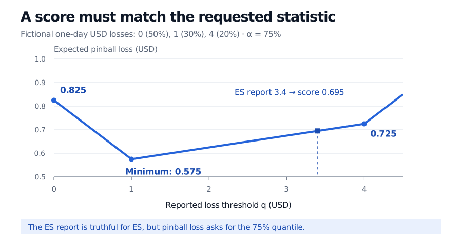
For fictional losses of USD 0, 1 and 4 with probabilities 50%, 30% and 20%, expected 75% pinball loss is minimised at report USD 1 with score USD 0.575. Scores at reports 0 and 4 are 0.825 and 0.725. Reporting ES of 3.4 gives score 0.695.
Original fictional example. The line shows expected score as the report changes, not a realised loss path. The ES report is truthful for a different target, so it need not minimise a quantile score.
For the weighted-average step, Expectation, Variance and Covariance develops expectation from discrete probabilities. Its public page is a preview; the full lesson requires a free signed-in account.
ES alone and ES alongside VaR
Expected shortfall averages the worst specified probability mass. Here the worst 25% contains all 20% at USD 4 and five percentage points of the mass at USD 1:
ES0.75=0.250.20(4)+0.05(1)=3.4 USD.
The strict-exceedance average E[L∣L>1]=4 selects only 20%, so it is a different statistic. Evaluating the ES report 3.4 with pinball loss gives 0.695, above the score at 1. That demonstrates a target mismatch; it does not prove that ES lacks every possible standalone score.
The impossibility result concerns ES as a single report on sufficiently rich distribution classes. Gneiting's Theorem 11 covers classes containing all finitely supported distributions on an interval. It is not a claim about every restricted family: on deterministic-loss distributions, for example, ES equals the loss itself and squared error elicits it.
However, the pair VaR and ES is jointly elicitable. Under finite first moments and unique relevant quantiles, suitable scores evaluate the two reports together, with upper-tail loss reports satisfying e≥v. The expected joint score is uniquely minimised at the true pair (v,e); it cannot in general be split into an independent VaR score plus an independent ES score. Fissler and Ziegel, Corollary 5.5, prove this using lower-tail notation; reversing the outcome sign gives the upper-tail convention here. Their 2019 correction, §2, preserves the result on the maximal sensible VaR/ES action domain.
What the property lets you conclude
For forecast comparison, use the same target, horizon, outcome convention, observations and chosen consistent score for competing methods. Averaging realised scores estimates an expected comparison; finite samples, tail scarcity and serial dependence still affect uncertainty. Different consistent scores can rank imperfect forecasts differently.
Calibration asks a different question: whether forecasts satisfy the relevant distributional restrictions, possibly conditional on available information. Winning a score comparison does not establish calibration, and ES's standalone non-elicitability does not make ES backtesting impossible. Fissler, Ziegel and Gneiting, pp. 2–3, distinguish model verification from comparative backtesting.
Elicitability also says nothing by itself about easy estimation, next-period accuracy or subadditivity. Aggregating portfolio risk and scoring a forecast are separate mathematical tasks.
Sources
Tilmann Gneiting (2011), Making and Evaluating Point Forecasts, §§2.2–2.3, §3.3 and §3.4, especially Theorem 11: strict consistency, quantile scores and the distribution-class scope of standalone ES non-elicitability.