Turn orthogonal variance contributions into an entropy-based diversification count, and distinguish factor choice, holdings count and inverse Herfindahl concentration.
Effective number of bets
The effective number of bets is a diversification score that expresses the concentration of a portfolio's risk exposures as an equivalent number of equally important bets. In an entropy-based implementation, a portfolio carrying most of its variance in one uncorrelated factor has a count close to one, even if it contains many securities. The practical question is how many risk sources matter at the current portfolio weights.
A number without its construction is incomplete. This article uses exponential Shannon entropy of normalized PCA variance contributions, following the unconstrained construction in Meucci's Managing Diversification, sections 2.1 and 3. Other concentration measures and other ways of constructing uncorrelated factors can give different counts.
First choose what counts as a bet
Suppose a vector of one-period simple returns R has finite covariance matrix Σ, and the portfolio has fixed beginning weights w. Its return is w⊤R. Use the full orthonormal eigenvalue decomposition
Σ=EΛE⊤,E⊤E=I,Λ=diag(λ1,…,λn).
The principal-component returns F=E⊤R are uncorrelated. Portfolio exposures in those coordinates are a=E⊤w, so the additive variance contributions are
ci=ai2λi,V=w⊤Σw=i=1∑nci.
For V>0, normalize them into shares pi=ci/V. They are nonnegative and sum to one, making them suitable inputs to a discrete entropy:
H=−i=1∑npilnpi,Nent=exp(H).
Use natural logarithms and the convention 0ln0=0. With n retained components, 1≤Nent≤n: a single nonzero share gives one; equal shares give n. Exponentiation converts entropy into the number of equal shares that would have the same entropy.
These are variance shares, not the eigenvalues normalized by their sum. The weights enter through ai2. Eigenvalues describe variation available in the return universe; exposures determine how much of that variation the particular portfolio holds. Nor should signed contributions from correlated assets be inserted blindly into the logarithm: they can be negative and do not provide the nonnegative distribution used here.
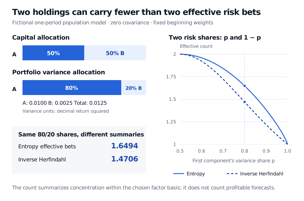
Two equally weighted assets: 1.6494 effective bets
Consider a fictional population model with two assets, one-period return variances 0.04 and 0.01, zero covariance, and 50% beginning capital in each:
Σ=(0.04000.01),w=(0.50.5).
The coordinate axes already form a PCA basis. All numbers are stipulated moments, with variance in decimal-return-squared units; there is no estimated return sample.
There are two holdings and two nonzero component exposures, but their unequal importance produces fewer than two equally important risk bets. The value 1.6494 is a continuous concentration summary; it does not identify a fractional security to trade.
Fictional two-asset model: capital weights 50/50 become variance shares 80/20, from contributions 0.0100 and 0.0025. Entropy effective bets equal 1.6494 versus inverse Herfindahl 1.4706. A curve compares both counts as the first risk share rises from 0.5 to 1; both decline from 2 to 1.
Original stipulated one-period population model. Shares refer to portfolio variance in the selected PCA basis. Solid line: exponential Shannon entropy; dashed line: inverse Herfindahl of the same shares.
For comparison, the inverse Herfindahl, also called a participation ratio in this use, is
N2=∑ipi21=0.82+0.221≈1.4705882.
It equals two for equal shares and one for full concentration, just as the entropy count does, but differs between those endpoints. State which formula and which shares are being reported. Applying either formula to capital weights would answer a different question.
The basis is part of the result
PCA selects statistical directions. Meucci, Santangelo and Deguest's minimum-torsion approach instead seeks uncorrelated factors that remain close to the original allocation factors. The author's lecture, PDF pp. 37–41, contrasts the resulting diversification profiles. The arithmetic above does not implement that optimization, and the PCA count should not be presented as a universal, basis-free definition.
Even PCA orientation can be ambiguous when eigenvalues repeat. In a second toy model, take Σ=0.01I and the same weights. The identity eigenbasis gives risk shares (0.5,0.5) and count two. A valid eigenbasis rotated so that its first axis is parallel to w gives shares (1,0) and count one, while total portfolio variance remains 0.005. Both bases diagonalize the same covariance. Record the orientation convention; nearly repeated estimated eigenvalues also deserve a stability check.
Comparisons therefore need a consistent factor universe, covariance horizon and estimation method, treatment of residual risk, normalization and portfolio weights. A count calculated after dropping components describes the retained risk, rather than automatically describing the entire portfolio.
Read the count alongside the risk
Multiplying all weights by the same nonzero constant multiplies every ci and V by its square, leaving the shares and count unchanged. The score can therefore remain unchanged while the magnitude of risk rises. Keep total risk and leverage beside it.
Uncorrelated factors need not be independent. This construction uses second moments; it does not rule out common downside events or make an out-of-sample loss guarantee. It also measures risk concentration rather than the number of successful alpha forecasts. A larger count alone says nothing about expected profit, trading costs or predictive skill.
Attilio Meucci, Managing Diversification, published in Risk 22(5), 2009, pp. 74–79; linked transcription of the 27 September 2010 revision. Section 2.1, equations (3)–(7): principal portfolios and variance shares; section 3, equation (18): exponential entropy count.
Attilio Meucci, (Re)Defining and Managing Diversification, university-hosted author lecture, PDF pp. 14–29 and 37–41: PCA construction, entropy and minimum-torsion comparison.