Compare time-series shapes with an explicit warping path, reproduce a zero-cost alignment, and understand cost conventions, timing constraints and real-time leakage.
Dynamic time warping
Dynamic time warping (DTW) compares two ordered sequences by finding a low-cost alignment that can stretch or compress their observation indices locally. In quant research, it can help retrieve historical time-series shapes that unfold at different speeds. The benefit comes with a choice: the method deliberately discounts some timing differences that may carry economic information.
For example, a volatility spike followed by a slow recovery might resemble a shorter spike-and-recovery episode after warping. That resemblance is a description of the selected observations and alignment rules. It does not establish that the episodes share a market mechanism or predict the same subsequent return.
What is allowed to move?
Take sequences x=(x1,…,xn) and y=(y1,…,ym). A warping path lists matched index pairs. Here it starts at (1,1), finishes at (n,m) and permits only the steps (1,0), (0,1) and (1,1). Neither index can go backwards or skip an observation. A horizontal or vertical step lets one observation match several consecutive observations of the other series.
Specify a local mismatch cost before optimising. This article uses
c(i,j)=∣xi−yj∣,DTW(x,y)=Pmin(i,j)∈P∑c(i,j).
There is no division by path length and no final square root in this definition. The minimum runs over the endpoint-anchored paths just described. Müller and Zalkow's DTW notebook develops this path formulation and an absolute-difference implementation.
A repeated value can cost nothing
Consider the fictional, dimensionless sequences
x=(1,2,3),y=(1,1,2,3).
Using one-based indices, an admissible path is
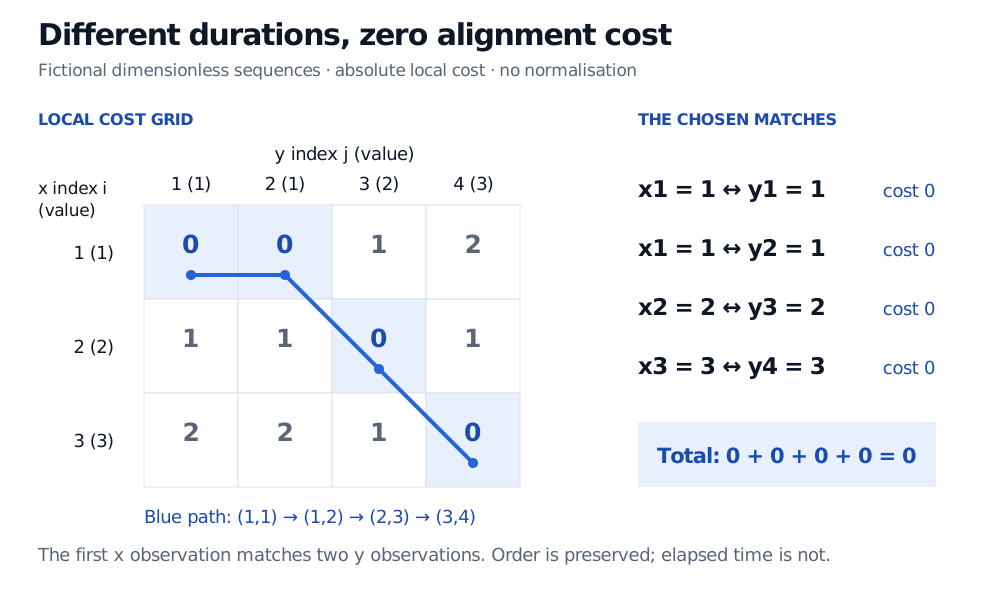
(1,1)→(1,2)→(2,3)→(3,4).
Its four matches compare 1 with 1, 1 with 1, 2 with 2 and 3 with 3. Every local cost is zero, so their sum is zero. Because all absolute costs are nonnegative, this path proves that the global minimum is zero.
Local absolute-cost grid for fictional sequences x=(1,2,3) and y=(1,1,2,3). The path (1,1), (1,2), (2,3), (3,4) visits four zero-cost cells, giving total DTW cost 0.
Original fictional example. The first observation of x matches both initial observations of y; the blue path preserves order while absorbing the repeated 1.
Zero DTW cost therefore does not mean identical sequences. Here even the lengths differ. Ordinary pointwise Euclidean distance requires an equal-length representation and a specified correspondence; it cannot be reported as zero for these two original vectors.
DTW is often called a distance, but it is not generally a mathematical metric. The zero-cost example already defeats the requirement that only identical inputs have distance zero. The triangle inequality can fail too. Under the same absolute-cost convention, let a=(0,0,1), b=(0,1,1) and c=(1,1,1). Then DTW gives d(a,b)=0, d(b,c)=1 and d(a,c)=2: the direct cost exceeds the sum through b. Do not assume a search or clustering method that requires metric properties remains valid unchanged.
Finding the path without trying them all
Let D(i,j) be the cheapest accumulated cost from the start through pair (i,j). Dynamic programming uses
D(i,j)=c(i,j)+min{D(i−1,j),D(i,j−1),D(i−1,j−1)}.
Initialise D(0,0)=0 and the rest of row zero and column zero to infinity. Fill the grid for positive indices; D(n,m) is the final score. Tracing an optimal predecessor backwards recovers a path. Ties can produce several optimal alignments.
The full grid has nm cells, giving an O(nm) computation for this recurrence. The small example has just 25 admissible paths, but exhaustive path enumeration becomes impractical as the sequences grow. The author notebook explains why the recurrence avoids that enumeration.
The constraints define the comparison
A warping band restricts which index pairs may be visited. For equal-length sequences, a Sakoe–Chiba band can impose ∣i−j∣≤r, where r is a maximum displacement in observations. A narrow band preserves more timing information; a wider band permits more deformation. With unequal lengths, state how the band is positioned and ensure that an endpoint-anchored path exists.
Sakoe and Chiba's original paper studies both window and slope restrictions. These limits can prevent a short segment from being stretched against a long, unrelated segment. They are modelling choices as well as computational controls; a lower unconstrained cost is not automatically a better economic comparison. Ratanamahatana and Keogh likewise examine the effect of constraint width rather than treating wider warping as universally preferable.
Other conventions change the result: squared differences instead of absolute differences, a square root after summation, direction-dependent step weights, path normalisation, or relaxed endpoints for subsequence search. A diagonal-only path under this article's absolute cost gives a sum of absolute differences. Under squared local costs followed by a square root, that diagonal-only score is Euclidean distance. “DTW score” alone is not a complete specification. Müller and Zalkow's variants notebook illustrates how step rules, weights and global constraints alter alignment.
Keep the market clock visible
Before a financial comparison, choose what the values represent: price levels, returns, volatility or another feature. Comparing raw levels retains scale differences; standardising each window removes some level and scale information. These answer different research questions. Scaling an incomplete live window using its eventual full-window mean and variance introduces look-ahead bias.
Keep the original timestamps alongside the path. Matching a one-day response to a ten-day response may help describe shape, while discarding the speed of repricing that matters for trading. Matching by observation index also does not resolve non-synchronous exchange closes or irregular event times. The Time-Series Data lesson covers timestamps, alignment and resampling; it has a public preview, with the full lesson requiring membership.
An offline alignment can use both completed windows. It cannot retrospectively become a signal available halfway through either window. At each simulated decision time, construct the query from the available prefix, search only information then available and recompute preprocessing within that boundary. The optimal alignment of a prefix can change when later observations arrive. A chronological, monotone path therefore does not by itself guarantee a causal real-time procedure.
Finally, choosing a window length, scaling method or band after seeing which historical analogue produced a favourable future return invites overfitting. Select these choices within earlier training/validation periods and assess the complete retrieval-and-decision procedure on later data. A visually persuasive match is a hypothesis to test, not evidence of a tradable edge.
Sources
Hiroaki Sakoe and Seibi Chiba (1978), Dynamic Programming Algorithm Optimization for Spoken Word Recognition, §II: warping functions, boundary/continuity restrictions, windows, slope constraints and alternative weighting conventions. The article's simple unnormalised cost is explicitly specified above; it is not a claim that every original-paper variant uses that convention.
Frank Zalkow and Meinard Müller, DTW Variants, FMP notebook: step sizes, local weights and global constraints.
Chotirat Ann Ratanamahatana and Eamonn Keogh (2004), Everything You Know about Dynamic Time Warping Is Wrong, §§2 and 4: DTW background and the role of warping-window constraints. Its dataset experiments do not establish financial forecasting performance.