Deciles mark tenths of a distribution. Distinguish nine cutpoints from ten ranked groups, calculate loss thresholds, and handle interpolation, ties and portfolio sorts.
Decile
A decile is a quantile at a multiple of 10%: the first decile is the 10th percentile, the second is the 20th, and so on through the ninth at 90%. These nine internal cutpoints describe ten ordered groups. In financial research, decile also means one of those groups: “the highest-loss decile” is a collection of observations, whereas “the ninth-decile loss” is a threshold in currency units. Statistics Canada's income-decile definition explicitly separates groups from their cutpoints.
For an increasing continuous distribution with cumulative distribution function F, the cutpoints satisfy F(Dk)=k/10, for k=1,…,9. Thus D5 is the median. For distributions with probability atoms, a generalised inverse provides a convention, for example Dk=inf{x:F(x)≥k/10}. The probability below a cutpoint need not then equal its nominal percentage exactly.
A loss report with twenty scenarios
Suppose a risk analyst has twenty equally weighted synthetic one-period loss scenarios, in USD:
x(1),…,x(20)=1,2,…,20.
The parentheses denote sorted positions, not dates. Positive values mean losses. No scenario probabilities for a real portfolio have been estimated here.
To report sample quantiles, the analyst must choose a calculation rule. Use R type 7 linear interpolation in this example. At probability p, set
h=1+(n−1)p,j=⌊h⌋,g=h−j,
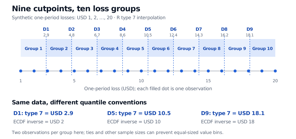
and interpolate as Q(p)=(1−g)x(j)+gx(j+1) for these interior probabilities. For n=20 and p=0.1, the position is h=2.9, giving D1=2+0.9(3−2)=USD 2.9. This is a location between observations, not a recorded loss. Type 7 is a named choice among the nine algorithms documented by R.
Cutpoint
Probability level
Type 7 result, USD
Interpretation in this sample
D1
10%
2.9
Losses 1 and 2 lie below it
D5
50%
10.5
Ten losses lie below it
D9
90%
18.1
Losses 19 and 20 lie above it
Here the highest-loss group contains 19 and 20, not every loss above D1. The threshold D9=18.1 is neither that group's average nor the worst loss. Its average is USD 19.5; the largest scenario loss is USD 20.
Twenty filled dots represent synthetic one-period losses USD 1 through USD 20. Nine type 7 cutpoints from USD 2.9 to USD 18.1 split them into ten groups of two. D1, D5 and D9 are USD 2.9, USD 10.5 and USD 18.1, compared with empirical inverse-CDF values USD 2, USD 10 and USD 18.
Original synthetic loss scenarios. Dashed lines are interpolated type 7 cutpoints; filled dots are observations. Groups are ordered from smaller to larger losses.
The algorithm and the grouping rule are separate choices
Another defensible convention takes the first observed value whose cumulative empirical proportion reaches p. With these twenty equally weighted observations, that empirical inverse-CDF rule gives x(⌈20p⌉): D1=2, D5=10 and D9=18, all in USD. Both sets of results use the same data. NIST describes several interpolation conventions and the absence of a universally accepted choice. Carry the method with the reported number.
To turn cutpoints into groups, state which group includes a boundary observation. One rule puts values at or below D1 in group 1, values strictly above D1 and at or below D2 in group 2, and continues through values above D9 in group 10. The figure has two observations per group because of its particular untied data and sample size.
Ten groups do not guarantee ten equal counts. If the sample size is not divisible by ten, equal integer group sizes may be impossible. Ties are a stronger obstacle: twenty identical losses give nine identical cutpoint values. Keeping equal losses together cannot produce ten nonempty value groups. A rank-based allocation may split tied records using an explicit secondary rule, but that rule adds no economic distinction between equal losses. Weighted data require cumulative weights rather than a silent assumption of equal counts.
Reading a decile portfolio table
A researcher might rank stocks by a signal and compare subsequent returns of the highest and lowest groups. First establish what “highest” means: high forecast return and high estimated loss point in different economic directions. Check whether decile 1 labels the lowest or highest ranks; tables use both conventions. Also check the eligible universe and whether ranking occurs within sectors or across all stocks.
A ranked basket becomes a strategy only after specifying information availability, formation and execution times, holdings, weights, rebalancing, and trading costs. A historical spread between group-average returns does not supply those choices or establish a future profit. The Portfolio sorts lesson develops sector rankings, weights and forward holding windows; the public page is a preview and the full lesson requires membership.