Cramér V: Definition & Examples

Cramér V is a dimensionless measure of association between two categorical variables, obtained by normalising Pearson's chi-squared statistic to a scale from zero to one. In a quant research audit, it can summarise how differently model assignments are distributed across market-regime labels. It measures the size of a categorical pattern; it does not tell you which model earns more or why the pattern exists.

From counts to association

Start with a two-way table of counts. Let $O_{ij}$ be the count in row $i$ , column $j$ , with $r$ rows, $c$ columns and total count $N$ . Under independence, the expected count is

E_{ij}=\frac{O_{i+}O_{+j}}{N},

where $O_{i+}$ and $O_{+j}$ are the row and column totals. The usual sample statistic is

\chi^2=\sum_{i=1}^{r}\sum_{j=1}^{c}\frac{(O_{ij}-E_{ij})^2}{E_{ij}}, \qquad V=\sqrt{\frac{\chi^2}{N\min(r-1,c-1)}}.

Use Pearson's statistic without a continuity correction for this conventional definition. SciPy's association function provides the corresponding nominal-association calculation. Here

V

denotes the empirical estimate; the population measure replaces cell proportions with population probabilities.

Remove unused categories with zero marginal totals before calculating. At least two nonempty rows and two nonempty columns are needed. A zero observed cell is allowed when its expected count is positive.

The dimension factor is $\min(r-1,c-1)$ , whereas the usual chi-squared test of independence uses $(r-1)(c-1)$ degrees of freedom. Those quantities answer different questions and must not be interchanged.

Two models, three regimes

Consider 100 fictional, independent cases, each classified once by the model assigned to it and once by its regime. The labels are categories, not numerical scores.

Assigned model	Regime 1	Regime 2	Regime 3	Total
A	30	10	10	50
B	10	20	20	50
Total	40	30	30	100

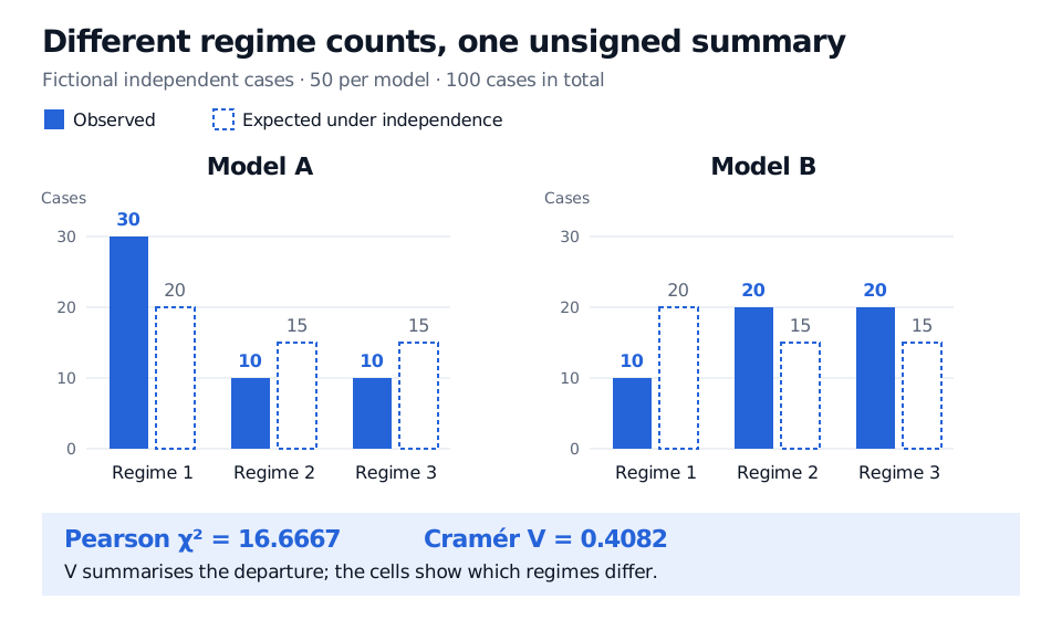
Independence would give expected counts 20, 15, 15 in each model row. Summing the six Pearson contributions gives

\chi^2=\frac{50}{3}\approx16.6667, \qquad V=\sqrt{\frac{50/3}{100\times1}} =\sqrt{\frac16}\approx0.4082.

Observed and expected counts for fictional independent cases: model A has regime counts 30, 10, 10; model B has 10, 20, 20. Each model has independence expectations 20, 15, 15. Pearson chi-squared is 16.6667 and Cramér V is 0.4082.

Original fictional example. Solid bars show observed counts; outlined bars show expectations from the same margins. The single V value compresses six cell departures.

The cells carry information that $V$ discards: 60% of A cases fall in Regime 1, compared with 20% of B cases. Renaming the regimes, swapping the model rows or transposing the table leaves $V$ unchanged. Inspect row proportions and cell departures to describe the pattern.

Unlike signed correlation,

V

cannot distinguish a positive relationship from a negative one. It also supplies no causal direction. The model could have been chosen because of the regime, or both classifications could reflect another variable. A value of 0.4082 is not 40.82% of variance explained, a forecast hit rate or a profit estimate.

Magnitude and significance travel separately

For this table, the usual asymptotic chi-squared reference has two degrees of freedom and yields a p-value of approximately 0.0002404. This assesses compatibility with independence under the sampling assumptions. It does not measure the pattern's economic importance.

Multiply every count by ten: the proportions and raw

V

stay the same, while

N

and

\chi^2

both multiply by ten. The asymptotic p-value falls. This is why an effect size and a significance test belong alongside each other. Repeating the original observations ten times would not create ten times as much independent evidence.

Sparse counts can make the asymptotic reference inaccurate; SciPy's chi-squared documentation discusses permutation and Monte Carlo alternatives. Serially repeated trades, overlapping outcomes or clustered instruments also require a sampling design that handles their dependence. Structural zeros require an appropriate model for the allowed cells. Computing a descriptive

V

does not repair these inference problems.

Which V did the report calculate?

Raw sample

V

can overstate population association through sampling noise, particularly with small samples and many categories. Bergsma's bias-correction paper, §2, proposes

\begin{aligned} \widetilde{\phi}^{\,2} &=\max\left(0,\frac{\chi^2}{N}-\frac{(r-1)(c-1)}{N-1}\right),\\ \widetilde r&=r-\frac{(r-1)^2}{N-1}, \qquad \widetilde c=c-\frac{(c-1)^2}{N-1},\\ \widetilde V &=\sqrt{\frac{\widetilde{\phi}^{\,2}}{\min(\widetilde r-1,\widetilde c-1)}}. \end{aligned}

This requires

N>1

and a positive corrected denominator. In the worked table,

\widetilde V=\sqrt{29/196}\approx0.3847

, compared with raw

V\approx0.4082

. Bias correction does not mean exact unbiasedness; truncating at zero leaves bias at population independence. It is also different from Yates' continuity correction, which modifies the chi-squared statistic for a one-degree-of-freedom table. Report the chosen convention explicitly.

Do not interpret a sample value of zero as proof of population independence. Nor should values from different category definitions be treated as automatically comparable: splitting regimes, changing margins or changing sample size can affect interpretation and estimation bias. Use the actual table, sampling uncertainty and the economic question to interpret magnitude; there is no universal weak/strong cutoff that establishes a useful trading result.

For a financial application of categorical tables, Performance Persistence and Survivorship Bias classifies funds as winners or losers across periods and introduces the cross-product odds ratio. That supplies a complementary way to describe a binary pattern; it is not a Cramér V derivation. The full lesson requires membership; a public preview is available.

Sources

SciPy, association: nominal-variable association, function arguments and relation to the phi coefficient; documentation checked 30 October 2026.
SciPy, chi2_contingency: Pearson statistic, expected counts, degrees of freedom, Yates correction and resampling alternatives; documentation checked 30 October 2026.
Wicher Bergsma, A bias-correction for Cramér's V and Tschuprow's T, author-hosted paper, §§1–2 and §3 discussion: population versus empirical association, finite-sample bias and corrected estimator. Published in Journal of the Korean Statistical Society 42 (2013), 323–328.

From counts to association

Two models, three regimes

Magnitude and significance travel separately

Which V did the report calculate?

Sources

Related terms

Correlation

Effect size

P-value