Coskewness and cokurtosis measure third- and fourth-order joint return moments. Follow a four-state calculation, distinguish index conventions and avoid excess-kurtosis and pricing mistakes.
Coskewness and cokurtosis
Coskewness and cokurtosis are third- and fourth-order cross-moments of returns. They describe how deviations from the means combine across assets, extending covariance beyond pairs of deviations. A portfolio's asymmetry and fourth moment depend on these joint quantities; knowing each asset's own skewness, kurtosis and ordinary correlation does not generally determine them.
For a risk desk, the distinction is practical: an asset can have a symmetric return distribution on its own yet change the asymmetry of a portfolio when combined with market exposure.
Name the indices before interpreting the number
Let X=Ri−E[Ri] be an asset's centred return and Y=Rm−E[Rm] the centred market return over the same horizon. Two useful unstandardised co-moments are
mi,mm=E[XY2],mi,mmm=E[XY3].
The first weights the asset's signed deviation by the squared magnitude of the market deviation. A negative value means the probability-weighted negative asset deviations dominate after this weighting. Both unusually positive and unusually negative market deviations receive positive squared weights, so this is not a downside-only statistic.
The second preserves the sign of the market deviation through Y3: same-sign asset/market deviations contribute positively and opposite-sign deviations negatively, with greater emphasis on large market moves. These descriptions concern the aggregate moment, not a rule that holds in every state.
There is a family of co-moments, rather than one universal number per pair of assets. In general,
mijk=E[XiXjXk],mijkl=E[XiXjXkXl].
Reordering the same factors leaves their product unchanged: mi,mm=mm,im. Changing which asset is repeated changes the quantity: E[XY2] need not equal E[X2Y], and E[XY3], E[X2Y2] and E[X3Y] are different fourth-order entries. Collecting all entries gives the coskewness and cokurtosis tensors, often stored as flattened matrices. Boudt and co-authors' notation connects these arrays to portfolio moments.
Here we use the explicitly declared, dimensionless convention
C3(i;m)=σXσY2E[XY2],C4(i;m)=σXσY3E[XY3],
where the standard deviations are strictly positive and the relevant absolute moments are finite. Finite third absolute marginal moments suffice for the third-order product; finite fourth marginal moments suffice for the fourth-order products. Unit-free does not make these Pearson correlations or impose correlation's bounds of −1 and 1.
Check a paper's convention before comparing coefficients. For example, Harvey and Siddique's direct coskewness measure, equation (11), uses an asset's market-regression residual, rather than simply its demeaned return as above. Conditional co-moments also depend on a specified information set; the example below is unconditional.
Four states make the signs visible
Consider this fictional population distribution, with four equally likely states for one matched holding period. The entries are already centred return deviations, measured in percentage points (pp).
State
Probability
Asset X (pp)
Market Y (pp)
XY2 (pp³)
XY3 (pp⁴)
A
1/4
−1
−2
−4
8
B
1/4
1
−1
1
−1
C
1/4
1
0
0
0
D
1/4
−1
3
−9
−27
Both means are zero. Using the population probabilities, not an n−1 sample correction,
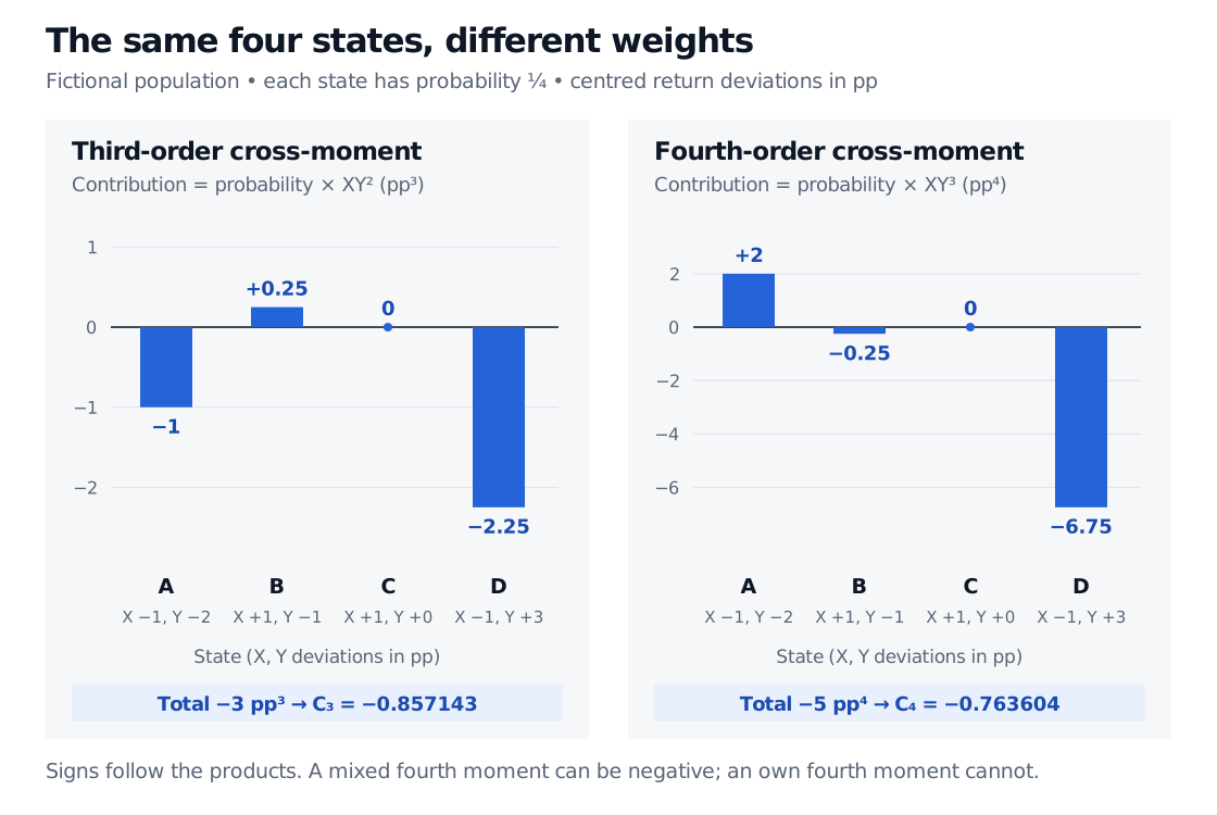
Probability-weighted contributions in four fictional equally likely states. For coskewness numerator XY squared, A contributes −1, B 0.25, C 0 and D −2.25 pp cubed, totalling −3. For cokurtosis numerator XY cubed, contributions are 2, −0.25, 0 and −6.75 pp to the fourth, totalling −5.
Original finite population model. Bars include each state's probability of one quarter; the two vertical scales have different units. State D dominates both negative totals, while state A contributes positively to the fourth-order total.
The asset alone has zero third central moment, because it takes −1 and 1 pp equally often. Nevertheless, its coskewness with the market is negative. Also E[X2Y]=0, because X2=1 pp2 in every state and E[Y]=0. The choice of repeated index matters even in this tiny model.
The negative cokurtosis is valid. Unlike an asset's own fourth central moment E[X4], a mixed product XY3 can be negative. This also differs from the nonnegative product X2Y2. Expressing both returns in decimals would change the unstandardised third and fourth moments to −3×10⁻⁶ and −5×10⁻⁸, respectively; the standardised coefficients remain unchanged.
Why portfolio construction needs the cross-terms
For fixed exposures a,b, put Z=aX+bY. Expanding its third central moment gives
Thus individual skewness and kurtosis cannot simply be averaged to obtain portfolio skewness and kurtosis. Compute the portfolio central moments using the joint distribution, then divide by the appropriate power of the portfolio's standard deviation if standardised measures are wanted. A negative individual cross-term does not make the complete portfolio fourth moment negative.
These marginal contributions also motivate asset-pricing models. Kraus and Litzenberger distinguish systematic skewness from an asset's total skewness; Harvey and Siddique develop a conditional model with exposure to squared market returns. A measured co-moment is an input to such a model. Its sign alone establishes neither a required return nor an investable risk premium, and the four fictional states supply no empirical pricing evidence.
Do not subtract three by habit
Ordinary excess kurtosis subtracts three from a variable's standardised own fourth moment. That adjustment cannot be transferred unchanged to every cross-moment.
For jointly Gaussian, centred X,Y with correlation ρ, the convention above has
E[XY3]=3Cov(X,Y)σY2,C4(i;m)=3ρ.
One can therefore define a Gaussian-benchmark excess cross-moment as C4(i;m)−3ρ, but that must be stated explicitly. Subtracting three applies to the own-moment case X=Y, where ρ=1; it is not an automatic cokurtosis convention. Neither coefficient in the worked example includes an excess adjustment.
Estimation is the difficult part
In historical data, a descriptive plug-in estimate replaces expectations with matched-date averages of centred products and uses a consistent variance convention. There is no universal n−1 correction that makes every standardised co-moment ratio unbiased. Record the return basis, market proxy, horizon, centring or regression model, weights and window alongside the estimate.
Powers magnify extreme observations. A short window may be dominated by a handful of moves; a long window may combine different regimes. Harvey and Siddique's later reassessment, §1, discusses estimation error and sensitivity to window and missing-value choices. Shrinkage toward a structured joint model can trade estimation variance for bias, as in Boudt and co-authors' §2.3; it does not make tail information plentiful.
A finite sample always produces finite arithmetic for finite observations, even when the population moments needed for the interpretation do not exist. Co-moments also summarise the entire distribution: they do not directly give a joint crash probability or tail dependence. Inspect scenarios and the joint return pattern alongside the coefficients.
For the probability-weighted calculations underlying this example, Expectation, Variance and Covariance develops centred products and portfolio variance. The public page is a preview; the full Mathematics Primer lesson requires a free signed-in account.