How the copper-gold ratio measures relative metal prices: quote-unit scaling, exact return arithmetic and limits of its macroeconomic interpretation.
Copper-gold ratio
The copper-gold ratio is the price of copper divided by the price of gold, using specified quote units and price series. It measures copper's relative price against gold. Macro researchers use it to explore industrial-demand conditions relative to demand for a perceived defensive asset; its movement alone does not identify the cause or forecast the next market move.
Read the units before reading the chart
Let Ct be copper quoted in USD per pound and Gt gold quoted in USD per troy ounce. Define
Qt=GtCt.
The resulting unit is troy ounces of gold per pound of copper: the amount of gold with the same quoted value as one pound of copper. The numerical level is therefore convention dependent. Current CME copper rules, §111102.C, specify dollars and cents per pound; gold rules, §113102.C, specify dollars and cents per troy ounce. Those are quote units, distinct from the quantity represented by a whole futures contract.
For a fictional, simultaneous pair of spot assessments with fixed metal specifications, take copper at USD 4 per pound and gold at USD 2,000 per troy ounce:
Q0=2,0004=0.002 troy oz/lb.
If copper is instead entered as 400 cents per pound, dividing the raw numbers gives 400/2,000=0.2. That is a different display convention, 100 times the previous numerical level. It does not mean copper became more expensive. Historical thresholds cannot be transferred between such charts without conversion. A rebased ratio index, 100Qt/Q0, removes a constant scaling factor; changing units halfway through the history creates an artificial jump.
Equal rallies cancel; unequal rallies do not subtract exactly
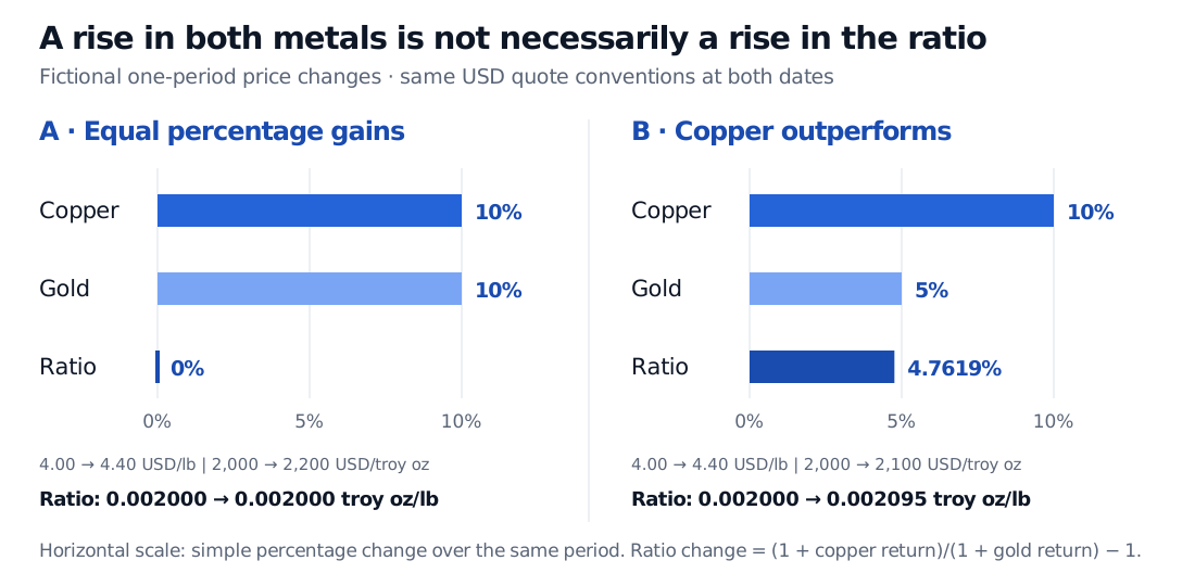
Keep those quote conventions and specifications unchanged. If copper rises to 4.40 and gold to 2,200, both gain 10% and the ratio remains 0.002. Rising industrial-metal prices alone do not establish a rising copper-gold ratio.
If copper instead rises to 4.40 while gold rises to 2,100, copper gains 10% and gold gains 5%. Now
Fictional one-period scenarios with copper in USD per pound and gold in USD per troy ounce: both gain 10% in scenario A and the ratio is unchanged; copper gains 10% and gold 5% in scenario B, so the ratio gains 4.7619%.
Original fictional one-period comparison. Bars show simple percentage changes, not current prices or portfolio returns; both scenarios begin at copper 4 USD/lb and gold 2,000 USD/troy oz.
For simple price returns rC and rG over the same interval,
Q0Q1−1=1+rG1+rC−1=1+rGrC−rG.
The 5 percentage point difference between the metals' returns is not the ratio's exact 4.7619% increase. For positive prices, the corresponding log change is exactly a difference:
log(Q0Q1)=log(C0C1)−log(G0G1)≈0.0465200.
Neither expression automatically describes a tradable portfolio's return. For example, hypothetical initial exposures of USD 100 long copper and USD 100 short gold would produce USD 10 minus USD 5, or USD 5 of price P&L, under the stipulated moves and before financing, borrowing and trading costs. A portfolio return still needs a capital denominator. Contract sizing, collateral and rebalancing rules cannot be recovered from the ratio chart.
A macro hypothesis with competing explanations
The industrial interpretation has a physical basis: the USGS copper overview describes uses in electrical infrastructure, construction, transport and machinery. Gold has a different demand mix, including jewellery, investment and central-bank reserves. That contrast motivates comparing the metals when researching the business cycle.
Jeffrey Mayberry's original DoubleLine discussion presents copper-gold as a macro dashboard indicator and proposes a relationship with the US ten-year Treasury yield. It also acknowledges misleading signals. That historical argument is a hypothesis to test for a stated sample and horizon, rather than a universal interest-rate equation.
A rise could reflect stronger copper demand, constrained copper supply, weaker gold demand, or several changes together. Conversely, gold demand can rise for reasons beyond immediate industrial activity. The ECB's June 2025 analysis examines official-sector and geopolitical demand and documents a breakdown after early 2022 in gold's earlier negative relationship with real yields. This illustrates why a fixed macro interpretation can fail. A ratio move establishes relative price performance; attributing it to growth, inflation or policy requires additional evidence.
What belongs in a research definition
A reproducible series identifies the two benchmarks, currency, metal specifications, observation times, frequency and quote scaling. A spot assessment and a deferred futures contract need not measure the same exposure. For futures histories, also specify delivery months, contract switches and adjustment rules: commodity roll yield explains why a maintained futures position differs from a spot-price change.
Converting both prices into the same new currency with the same contemporaneous exchange rate cancels that exchange rate in the ratio algebra. It does not remove currency influences on supply, demand or price formation. Mismatched currencies or observation times do not enjoy that cancellation.
Finally, state whether a model uses the ratio level, its change, or a rolling transformation. Fit transformations using information available at each decision time to avoid look-ahead bias, and evaluate the chosen forecast horizon on later data. A historical correlation supplies neither a causal explanation nor a ready-made trading rule.
For the market mechanics behind the inputs, the Commodities lesson explains physical specifications, storage, convenience yield and basis risk. Its public preview is open; the full lesson requires a free signed-in account.