Cohen kappa compares categorical agreement with a marginal-frequency benchmark. Work through 100 paired labels, prevalence effects and the separate weighted variant.
Cohen kappa
Cohen kappa (κ) measures agreement between two labelers on the same cases, adjusted for a benchmark formed from each labeler's category frequencies. A quant team might use it to audit whether two analysts apply a market-event labeling rule consistently before those labels become model inputs. Agreement alone cannot establish that the labels describe the market correctly.
Seventy agreements are not a kappa of 0.70
Two fictional analysts independently label the same 100 news events “yes” or “no” for a specified event category. Neither analyst is designated as the truth.
Analyst A / Analyst B
Yes
No
A total
Yes
40
10
50
No
20
30
50
B total
60
40
100
The diagonal contains 70 agreements, so observed agreement is po=0.70. A assigns “yes” half the time; B assigns it 60% of the time. Multiplying their respective marginal distributions gives the benchmark
pe=(0.50)(0.60)+(0.50)(0.40)=0.50.
Kappa compares agreement above that level with the remaining distance to perfect agreement:
κ=1−pepo−pe=1−0.500.70−0.50=0.40.
The result means the observed agreement covers 40% of the gap from this benchmark to perfect agreement. It does not mean that 40% of labels are correct. The formula and separate labeler-frequency convention are described in scikit-learn's kappa reference.
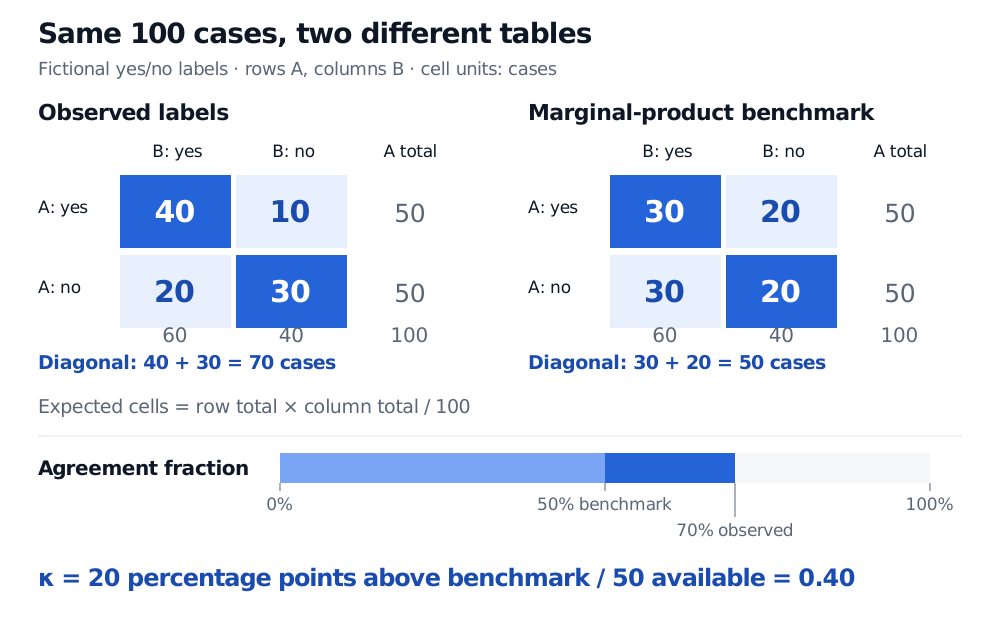
Two fictional analysts label 100 cases. Observed rows are 40 yes/yes and 10 yes/no, then 20 no/yes and 30 no/no. Marginal-product expected rows are 30 and 20, then 30 and 20. Observed agreement 70%, benchmark 50%, and kappa 0.40.
Figure: The benchmark preserves both analysts' category totals but replaces the observed pairing with marginal products. Blue diagonals count agreement; the lower bar shows the 20 percentage points above the 50% benchmark.
What “chance” specifies
For K mutually exclusive, exhaustive categories, let nij count cases assigned category i by A and j by B. With n paired cases, write ri=ni+/n and ci=n+i/n for the row and column proportions. Then
po=n∑i=1Knii,pe=i=1∑Krici.
The products describe a hypothetical independence benchmark with those marginal frequencies. Computing pe does not demonstrate that the real labelers guessed randomly or worked independently. Independent labeling is a study-design choice; statistical independence is the benchmark's factorization. Shared instructions, shared information and case difficulty can still produce dependent labels.
Cohen's own retrospective explanation motivates why the expected agreement depends on how often each category is used. Here, “chance-adjusted” names a specific convention, rather than a uniquely determined correction for every labeling process.
An equivalent reading uses disagreement:
κ=1−1−pe1−po.
In the example, 30% observed disagreement is 60% of the benchmark's 50%, leaving κ=0.40. Zero means agreement equals the benchmark; a negative value means agreement is below it. If pe<1, perfect agreement gives one. If both labelers assign every case to the same single category, po=pe=1: the ratio is undefined, despite 100% raw agreement.
Prevalence changes the comparison
Keep raw agreement at 90%, but change the category totals. These are two further fictional datasets, each containing 100 cases with rows A yes/no and columns B yes/no:
Dataset
A-yes row: B yes, B no
A-no row: B yes, B no
po
pe
κ
Balanced label frequencies
45, 5
5, 45
0.90
0.50
0.80
Both mostly say yes
85, 5
5, 5
0.90
0.82
4/9≈0.444
In the second dataset, each labeler uses “yes” on 90% of cases, giving pe=0.92+0.12=0.82. The same observed agreement now exceeds a much higher benchmark. Different marginal frequencies between labelers also affect pe; unequal row and column totals can prevent perfect agreement altogether. Report the table and both marginals alongside kappa, especially when comparing samples with different category prevalence. Artstein and Poesio, §3 analyze these marginal and prevalence effects.
Weighted kappa asks a different question
Ordinary kappa counts every off-diagonal pair as an equal disagreement. If categories have a meaningful order—say low, medium and high—one may instead choose weighted kappa. With observed proportions qij=nij/n and predeclared disagreement weights dij, a common convention is
κw=1−∑i,jdijricj∑i,jdijqij,
provided the denominator is positive. Set dii=0 and all off-diagonal weights to one to recover ordinary kappa. For equally spaced ordinal categories, linear weights can use dij=∣i−j∣/(K−1); quadratic weights square that distance. Category order and spacing now matter. Arbitrarily sorting nominal labels does not create a defensible distance scale. State whether supplied weights measure agreement or disagreement: software conventions differ. The statsmodels reference documents its score-distance weighting choices.
Agreement is one part of a label audit
Kappa is symmetric in the two labelers. Accuracy assigns a different role to one set of labels: it is a reference against which predictions are judged. Two analysts can share the same mistaken rule and agree perfectly; kappa supplies no external validation. If a trustworthy reference exists, inspect class-specific errors and their consequences. The membership lesson Evaluating Classifiers: Precision, Recall, and ROC/AUC develops that complementary analysis; its public page previews the full lesson.
Avoid treating verbal bands such as “fair” or “good” as universal acceptance rules. Specify the task, label definitions, paired-case selection, marginals, weighting and intended use. A sample kappa also has uncertainty: report a suitable confidence interval when making population claims. Repeated assets or overlapping time windows need an uncertainty method that respects their dependence; merely counting every label pair as an independent case can overstate precision. No interval is calculated for the fictional tables here.