Measure standard deviation relative to a positive mean, see why changing units preserves CV, and recognise the limits of near-zero means and return comparisons.
Coefficient of variation
The coefficient of variation (CV) is standard deviation divided by the mean. It measures spread relative to the average level. For a quant comparing positive execution costs or processing times, it can separate a large absolute spread from a large relative spread—but only when the measurement has a meaningful zero and the mean is safely positive.
The units cancel. A CV of 0.2, often reported as 20%, means the standard deviation is one fifth of the mean. It is neither a probability nor the fraction of observations outside a particular interval. NIST's definition emphasises this relative-dispersion interpretation and the measurement-scale restriction.
Three costs, two different kinds of transformation
Take three fictional observed transaction costs: 8, 10 and 12 USD, measured on the same basis. Zero USD means no cost. Treat them as a sample and use the n−1 standard-deviation convention:
xˉ=10,s=3−1(8−10)2+(10−10)2+(12−10)2=2.
Therefore the sample CV is s/xˉ=2/10=0.2=20%.
Representation
Mean
Sample SD
CV
Original costs: 8, 10, 12 USD
10 USD
2 USD
20%
Same costs: 800, 1000, 1200 cents
1000 cents
200 cents
20%
Add 100 USD to every cost: 108, 110, 112 USD
110 USD
2 USD
About 1.82%
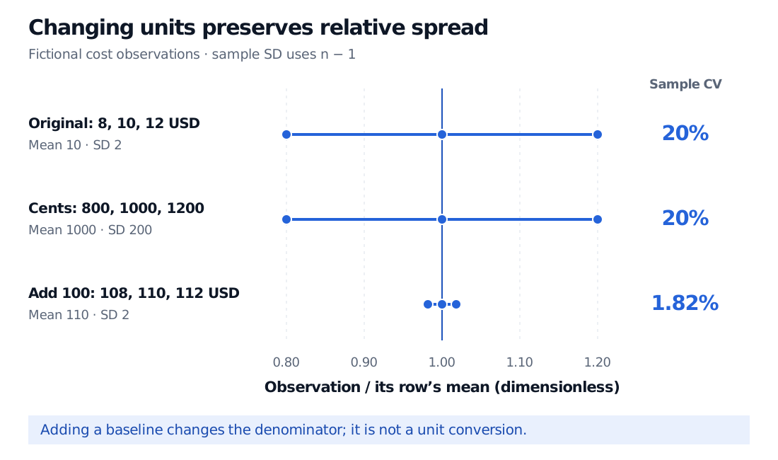
Converting dollars to cents multiplies both mean and SD by 100, leaving CV unchanged. Adding a constant changes the mean but leaves SD unchanged: the last row gives 2/110=1/55≈1.818%. That row describes different costs, rather than another unit for the original costs. Its lower CV does not mean smaller dollar fluctuations.
Fictional costs 8, 10 and 12 USD have mean 10, sample SD 2 and CV 20%. Converting to 800, 1000 and 1200 cents preserves CV 20%. Adding 100 USD gives mean 110, SD 2 and CV about 1.82%. Points are divided by each row mean.
Original fictional observations. A common change of units preserves the spacing relative to the mean; adding a constant compresses that relative spacing without changing the USD standard deviation.
This distinction explains ratio scale: ratios such as “twice the cost” must have a stable meaning, with zero representing absence of the measured quantity. A unit conversion multiplies all observations by a positive constant; it does not move the origin. CV survives the former but changes under the latter. An arbitrary baseline can therefore manufacture a different CV. Celsius temperature is a standard counterexample; its zero is not absence of temperature. The GraphPad statistics guide explains this measurement-scale distinction.
The variance of the original sample is 4 USD2; its SD is 2 USD; its CV is dimensionless. These are distinct statistics. Also state the divisor: treating the three observations as an entire equally weighted population gives SD 8/3≈1.633 USD and CV about 16.33%, rather than 20%. SciPy's official definition and ddof documentation illustrate why a software default must be checked. Using n−1 for variance does not make the resulting ratio an unbiased estimator of population CV.
A small denominator can dominate the story
At a zero mean, division by the mean is undefined. Near zero, a small change in the estimated mean can produce a huge change in CV even when absolute spread barely changes. For example, observations −1.9, 0.1 and 2.1 have sample SD 2 and mean 0.1, giving CV 20, or 2000%. This is a denominator warning, not evidence of a precisely measured economic risk multiple.
A negative mean produces a negative value under the signed definition s/xˉ. It does not imply negative dispersion or superior stability. Replacing the denominator with ∣xˉ∣ defines a different convention and still does not fix instability near zero. NIST distinguishes an absolute-denominator relative standard deviation from signed CV; SciPy likewise documents its signed calculation.
For positive quantities, CV can complement the mean and SD. It cannot reveal tail shape, dependence or estimation uncertainty, and there is no universal “good CV” cutoff. Three illustrative costs establish the arithmetic, not a reliable estimate of an execution-cost distribution.
Returns need an explicit benchmark
Raw investment returns can have small or negative means, making a casual CV ranking particularly fragile. Nor is their CV automatically the inverse Sharpe ratio. Sharpe's original discussion uses the mean and SD of differential returns relative to a benchmark.
With a constant risk-free return rf, one-period Sharpe is (Rˉ−rf)/sR. For stipulated same-period mean return 6%, SD 12% and risk-free return 2%, raw-return CV is 12/6=2, but Sharpe is (6−2)/12=1/3, rather than 1/2. Only with explicitly zero risk-free return, nonzero mean and SD, and the same observations, horizon and SD convention does raw-return CV invert that Sharpe calculation. Equivalently, a CV calculated on the very same excess-return series is algebraically reciprocal when both ratios exist; its positive-mean interpretation remains conditional.
For the underlying quantities, Expectation, Variance and Covariance develops means and dispersion from a worked return model. The full primer lesson is available with a free signed-in account; its public page provides a preview.
Sources
NIST Dataplot, Coefficient of Variation, Description and Note: ratio-scale meaning, sensitivity near zero, and the absolute-denominator relative-SD convention.
SciPy, scipy.stats.variation, definition, ddof and Notes: signed mean, sample-SD divisor and zero-mean behaviour.