The sure return that matches a risky return’s expected utility, with an exact exponential-utility example, mean–variance limits and explicit return-versus-wealth conventions.
Certainty-equivalent return
A certainty-equivalent return is the sure return that gives the same utility as an uncertain return over a stated horizon. It translates a return distribution into a rate under specified preferences. In portfolio construction, it makes the trade-off explicit: how much expected return would this decision maker give up to remove this particular risk?
Unlike expected return, the certainty equivalent depends on both the distribution and the utility function. Two investors can agree on every possible outcome and probability yet assign different certainty-equivalent returns.
First fix what utility measures
For initial wealth W0>0, one-period simple return r produces final wealth W0(1+r). Under expected utility, the certainty-equivalent return c solves
u(W0(1+c))=E[u(W0(1+r))].
Equivalently, define return utility U(r)=u(W0(1+r)). Then
c=U−1(E[U(r)]).
The inverse acts after averaging utility. Averaging returns first and then applying utility answers a different question. Assume U is continuous and strictly increasing, and that the expectation exists and lies in its range. For increasing concave utility, c≤E[r]; strict concavity gives a strict inequality for a nonconstant bounded return. The gap E[r]−c is the utility-based risk premium in return units. It is a preference valuation, not a realised loss or the market's equilibrium excess return.
A 5% mean can be worth 3.52197% for certain
Consider a fictional one-period lottery with simple returns −5% or +15%, each with probability one-half. Stipulate utility directly over decimal returns:
U(r)=−e−γr,γ=3.
Here r=−0.05 or 0.15, and γ is 3 per decimal return unit. This is constant absolute risk aversion in the return variable. It is not a dimensionless CRRA coefficient of 3 applied to final wealth. Writing returns as percentage-point numbers, −5 and 15, would require coefficient 0.03 to preserve the same preferences.
The variance uses the stipulated population probabilities:
Thus the lottery and a sure 3.52197% return have equal utility under these preferences. The gap from the 5% mean is approximately 1.47803 percentage points. This does not mean the lottery will realise 3.52197%; its only outcomes remain −5% and +15%. The example specifies a preference model, not an investment recommendation.
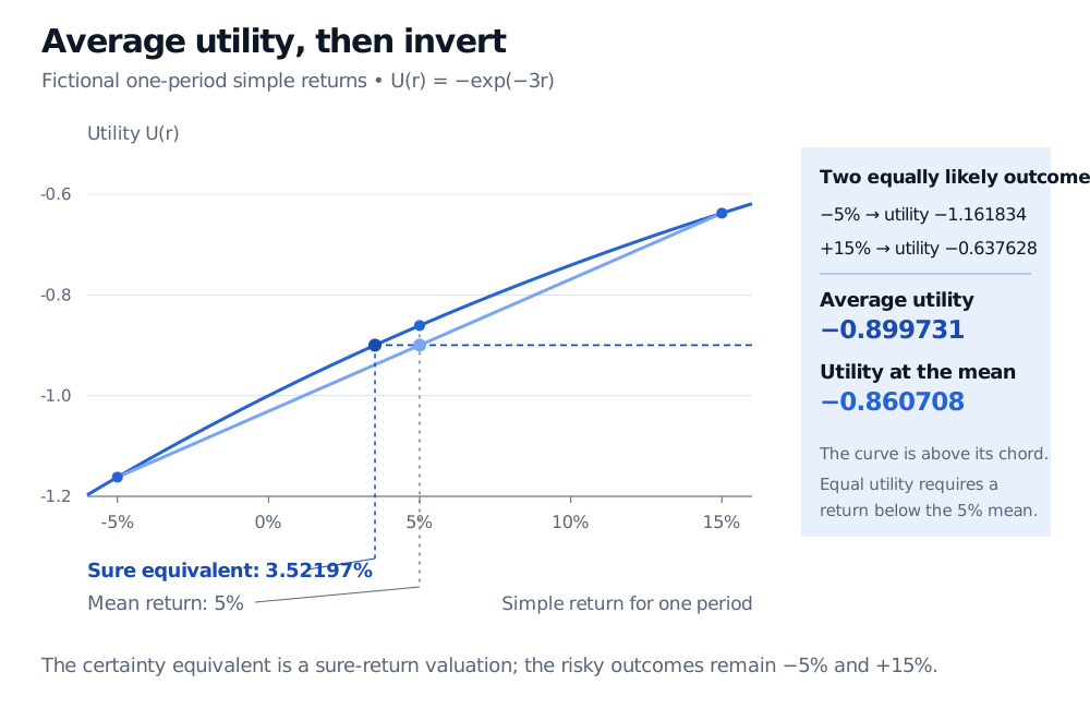
A fictional two-outcome return lottery under U(r)=-exp(-3r). The equally likely −5% and +15% returns have mean 5%. Average utility is −0.899731, equal to utility at the sure return 3.52197%; utility at the mean is higher, −0.860708.
Original fictional example. The straight chord averages the two utilities. Its midpoint sits below the utility curve at the mean; moving horizontally to the curve identifies the certainty equivalent.
When the mean–variance expression is exact
For exponential return utility, the exact formula is
c=−γ1logE[e−γr].
A second-order expansion for a small spread of returns around their mean gives
c≈μ−2γσ2.
In the lottery above, this is 0.05−(3/2)(0.01)=0.035, or 3.5%. It understates the exact certainty equivalent by about 2.20 basis points. The closeness here does not make it an identity for two-point distributions; more generally, the exponential expectation depends on the whole distribution and can fail to be finite for a sufficiently heavy left tail.
There is an exact special case. If r has a normal distribution with mean μ and variance σ2, then
E[e−γr]=e−γμ+γ2σ2/2,c=μ−2γσ2.
This exponential-utility/Gaussian combination supplies a utility foundation for mean–variance optimisation. An unbounded Gaussian simple return can fall below −100%, so its economic suitability still depends on the position being modelled. The algebra being exact does not validate the return model.
SelfMadeQuant's Mean–Variance Optimisation develops the quadratic portfolio objective, constraints and risk-aversion trade-off. A public preview is available; the full lesson requires membership.
Changing utility changes the answer
Exponential utility of wealth, u(W)=−e−aW, induces exponential return utility with γ=aW0, up to a positive constant multiplier. Holding the wealth-utility coefficient a fixed while changing initial wealth therefore changes the effective return coefficient. A return-based parameter cannot be moved to a wealth-based calculation without this conversion.
For positive final wealth, CRRA power utility instead gives, for relative risk aversion η>0 and η=1,
c=(E[(1+r)1−η])1/(1−η)−1.
Its log-utility limit is c=exp(E[log(1+r)])−1. These formulas require 1+r>0 and the relevant finite expectations. They are different preference models from the exponential example; the mean–variance expression is generally only a local approximation for them.
Compare certainty equivalents using the same horizon, simple-versus-log convention, probabilities, starting-wealth treatment and utility parameters. A certainty equivalent for one period cannot be annualised mechanically without specifying the joint return and compounding model. It is also distinct from utility indifference pricing, which finds a transaction price by comparing optimised utility with and without a claim. There is no universal certainty-equivalent “risk-adjusted return” independent of those choices.
Sources
Alexander Wolitzky, Attitudes toward Risk, MIT 14.121, Fall 2015, slides 2–11: expected utility, certainty equivalents, concavity and absolute versus relative risk aversion.
Bengt Holmstrom, Lecture Slides — Part 2, MIT 14.124 course materials, slides dated 2 February 2016, slides 34–36: exponential utility, normal noise and the mean–variance certainty equivalent. The return lottery, unit conversions and derivations above are independently worked.