Weight normalisation separates a neural-network weight vector into direction and learned scale. See the geometry, gradient changes and distinction from activation normalisation.
Weight normalisation
Weight normalisation is a reparameterisation of a neural network that learns a weight vector through separate direction and scale parameters. For a financial prediction model, it offers a way to change training geometry without making an observation's forward calculation depend on the other observations in its mini-batch. It does not standardise the financial inputs.
A direction, then a scale
For one neuron's incoming weight vector, write
w=g∥v∥2v,v=0.
The vector v/∥v∥2 has unit Euclidean length. The scalar g controls scale; the bias remains a separate parameter. Training updates v and g, differentiating through this expression, rather than updating w and normalising it afterwards. This is the method introduced by Salimans and Kingma (2016), §2.
If g is allowed to be signed, the precise identity is ∥w∥2=∣g∣. A nonnegative parameterisation makes g the length itself. Either way, a learned scale is not a fixed norm constraint: the weight norm can grow or shrink during training. The expression is undefined at v=0.
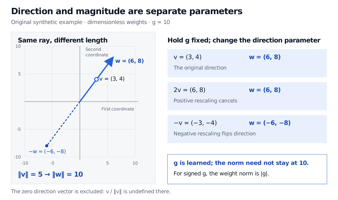
Take the synthetic, dimensionless parameters v=(3,4) and g=10. The direction parameter has length 5, so
∥v∥2v=(0.6,0.8),w=(6,8),∥w∥2=10.
Doubling v to (6,8) leaves w unchanged: its numerator and denominator both double. Replacing v by (−3,−4) instead gives w=(−6,−8) when g stays at 10. To preserve the original weight vector after that sign reversal, also change g to −10.
Synthetic dimensionless example: direction parameter v is (3,4), with length 5, and g is 10, producing w equal to (6,8), with length 10. Doubling v leaves w unchanged. Negating v with fixed g gives w equal to (minus 6, minus 8).
Original synthetic geometry and parameter comparison. Positive rescaling of the direction parameter cancels; negative rescaling changes the represented direction unless the scale also changes sign.
Same predictions, different optimisation coordinates
At any fixed represented weight w, the neuron computes the same prediction as before. The change lies in how a loss gradient reaches its trainable parameters.
Let u=v/∥v∥2 and let h=∇wL. The chain rule gives
∂g∂L=u⊤h,∇vL=∥v∥2g(h−u(u⊤h)).
The direction gradient removes the component along u and rescales the remainder. This explains how changing coordinates can change an optimiser's trajectory even while representing the same family of weight vectors; see the paper's gradient derivation, §2.1.
For the example above, suppose a local loss has h=(1,0). Then ∂L/∂g=0.6 and ∇vL=(1.28,−0.96). The direction gradient's dot product with v is 3(1.28)+4(−0.96)=0. That orthogonality is a local derivative property, not a guarantee that a finite update leaves ∥v∥2 unchanged. Nor does it guarantee nonvanishing gradients elsewhere in a deep network.
Which object is being normalised?
Batch normalisation and layer normalisation transform activations. Weight normalisation transforms the parameters used to produce them. Pure weight normalisation needs no running activation mean or variance, and no training-versus-inference switch for batch statistics. Adding a batch-dependent layer to the same network changes that statement about the whole model.
Initialisation still matters. The original paper's optional data-dependent initialisation estimates activation statistics from an initial batch; that is distinct from the ongoing weight reparameterisation. For a chronological financial experiment, using a future evaluation period for such initialisation would introduce preprocessing leakage. Weight normalisation itself does not repair that research design.
In PyTorch, the parametrisation API defaults to an independent norm per output channel with dim=0; dim=None uses the entire weight tensor. These define different normalisation groups. The older torch.nn.utils.weight_norm API is deprecated in favour of that parametrisation API. Check the chosen axis and saved model representation when reproducing a model.
For the surrounding research process, Mini-Batches, Vectorization, Autograd, and a Reproducible MLP Workflow connects automatic differentiation with chronological splits, training-only preprocessing and saved checkpoints. Its public page is a preview; the full lesson requires membership. Whether the reparameterisation helps a particular financial model remains an empirical question for that evaluation process.