Aggregated search queries can measure attention before economic releases, but sampling, relative scales, query definitions and historical vintages shape the signal.
Web search data
Web search data records how often people submit particular queries to a search engine, usually aggregated by time and geography. In quant research, it is a form of alternative data that can supply a timely measure of attention or purchase planning. Its usefulness depends on what the provider actually reports: a query count, a share of searches or a rescaled interest index have different meanings.
A search for a retailer does not establish a visit or a purchase. Someone might be comparing prices, seeking a refund or reading news about the company. Website traffic measures visits to destinations; app usage data measures activity within apps. Search data measures the act of asking the search engine, including searches that never produce either kind of visit.
What does 100 mean?
Google Trends is a familiar example, but its website does not expose an absolute query-count series. Google's data FAQ describes sampled, anonymised and aggregated searches. It divides search activity by total searches for the relevant geography and time, then rescales relative interest to a 0–100 range. Equal indices in different regions need not represent equal numbers of searches.
To isolate the rescaling effect, consider a fictional one-term dataset with exactly 1,000 total searches in every time bucket. This fixed denominator makes counts proportional to query shares. A simplified peak-normalised index is
st=Ntct,It=100maxu∈Wsust,
where ct is the query count, Nt is all searches in that bucket, and W is the comparison window. This teaching calculation omits sampling, rounding, filtering and privacy noise; the counts below are invented, not recovered Google counts.
Fictional request
Query counts by bucket
Query shares
Rescaled indices
Window A
20, 40, 10
2%, 4%, 1%
50, 100, 25
Window B
20, 80
2%, 8%
25, 100
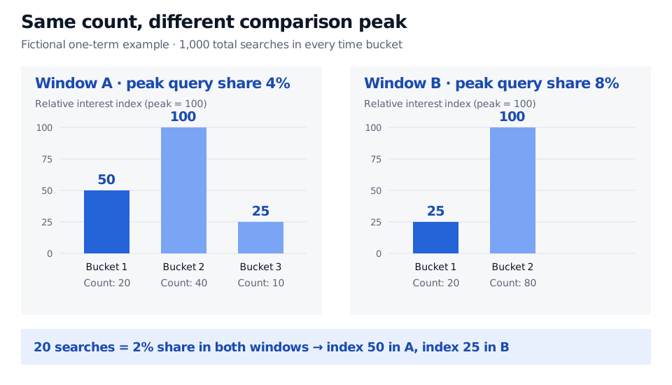
The count of 20 is unchanged. Its share is also unchanged at 2%. Yet its index is 50 in A and 25 in B because the comparison peak changes. Pasting independently scaled downloads together can therefore manufacture a discontinuity. A value of 100 means the comparison's peak relative interest; it does not mean 100 searches or that everyone searched.
Fictional Window A counts 20, 40 and 10 become indices 50, 100 and 25; Window B counts 20 and 80 become 25 and 100. Every bucket contains 1,000 total searches. The count of 20 has index 50 in A and 25 in B.
Original fictional fixed-denominator example. The two comparison windows have separate peaks; the raw counts are stipulated for teaching and are not visible Google Trends volumes.
The denominator matters too. If the query count stays at 20 while total searches rise from 1,000 to 2,000, query share falls from 2% to 1%. A decline in relative interest can therefore occur without a decline in the number of queries. Multiplying a Trends index by a guessed constant does not generally recover raw search demand.
This warning is specific to the measurement interface. As checked on 1 November 2026, Google's API alpha page still describes application-based, limited access and consistently scaled data across requests. Its July 2025 announcement explicitly says those API values remain search interest, rather than absolute counts. Cross-request consistency addresses the website's request-by-request scaling problem; it does not turn the result into a census of queries.
Define the query before testing the signal
A company name can be ambiguous. “Apple” may concern fruit, a device, a repair or a share price. Google's comparison guide distinguishes terms, matched under its term rules, from topics, which group expressions referring to a concept across languages. It also distinguishes an ordinary multiword term from an exact phrase in quotation marks. A topic and a literal query are different measurement choices, even when their chart labels look similar.
Record the exact term or topic identifier, language treatment, category, search property, geography, time window, bucket frequency and timezone. Keep these settings with each export. Otherwise a change in the resulting feature might come from a changed request rather than changed behaviour.
Interpret small values carefully. Google's current FAQ says low-volume terms can appear as 0, and explains that privacy-related statistical noise can create apparent spikes for low-interest queries. A zero is not proof that nobody searched; a small isolated spike is not evidence of an identifiable person's search. Searchers also need not represent the population whose spending or employment the model aims to predict. That mismatch is a potential selection bias.
Preserve the information available at the forecast date
A search can precede an economic release without predicting a later economic period. Choi and Varian's Predicting the Present with Google Trends, in its December 2011 working-paper version, motivates nowcasting: using queries observed during a month to estimate that month's activity before the official report arrives. It treats prediction of later periods as a separate question. Its examples support investigating search data, rather than a guarantee that any keyword improves forecasts or predicts returns.
A historical observation date is not an availability timestamp. Preserve each downloaded vintage, retrieval time, request settings and any incomplete-period flag supplied by the provider. A download obtained today cannot, on its own, establish what an earlier researcher could have used. Later sampling, processing or a changed comparison window can alter the historical series returned. The owned Point-in-Time Data lesson develops historical version selection and snapshot audits. A public preview is available; the full lesson requires membership.
The peak issue has a precise qualification. A later, higher peak rescales earlier values in the toy example, so that newly normalised history was unavailable earlier. A model invariant to a common multiplicative rescaling might produce identical predictions, but thresholds, independently joined windows and rounded values need not. Preserve the actual historical input rather than assuming invariance repairs every look-ahead bias.
Evaluate a frozen query definition against a baseline using successive forecast origins and only then-available target releases. Choose terms and fit seasonal adjustments within the training process. Trying many keywords on the full outcome history and retaining the best creates data snooping. Finally, distinguish forecasting activity from making money: prices may already incorporate the information, and a tradable strategy still needs a timing rule, execution assumptions and costs.
Hyunyoung Choi and Hal Varian, Predicting the Present with Google Trends, working paper dated 18 December 2011, introduction and §§2–3.1. The numerical example and figure above are original.