TimeGAN combines latent-space adversarial generation with supervised temporal learning. A scalar example shows what its next-step loss measures and what it cannot validate.
TimeGAN
TimeGAN is a time-series generative adversarial framework that combines a learned latent representation with supervised learning of temporal transitions. For a quant researcher, its attraction is synthetic sequences that aim to preserve relationships across time, rather than merely plausible individual observations. Yoon, Jarrett and van der Schaar introduced it at NeurIPS 2019. Original paper, Introduction
Three learning signals
A generative adversarial network learns through competition between a generator and a discriminator. TimeGAN adds reconstruction and next-step supervision to that competition:
Component
Role
Embedding network
Encodes observed sequences into latent representations.
Recovery network
Maps latent sequences back to observed feature space. Together with the embedder, it forms an autoencoder.
Generator
Converts random inputs into synthetic latent sequences.
Discriminator
Distinguishes encoded real sequences from synthetic ones.
Reconstruction encourages the representation to retain information. Adversarial learning encourages realistic sequences. Supervision gives an additional signal about transitions between adjacent latent states. The embedding is learned jointly with temporal supervision, rather than being a fixed preprocessing step. Original paper, §4
The authors' released implementation separates out a fifth network, the supervisor. It predicts the next latent state from preceding latent information. For generation, its output transforms the generator's latent sequence before recovery produces synthetic observations. Training compares supervisor predictions on encoded real data with the real latent sequence shifted forward by one step. Thus the paper's four conceptual functions and the code's five named networks describe different levels of decomposition. Authors' implementation, network definitions and supervised loss
A supervisor can be right on two transitions
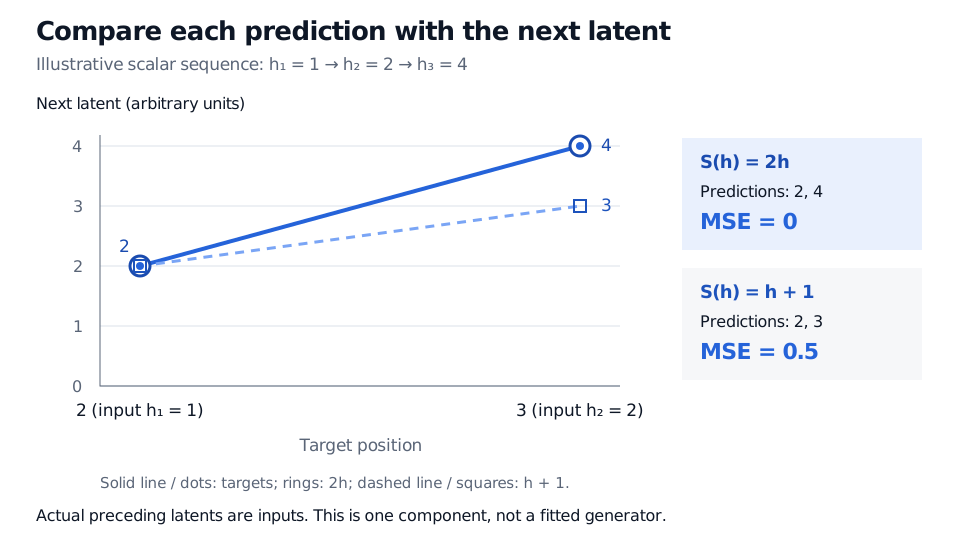
Take the illustrative scalar latent sequenceh1=1, h2=2, h3=4. These are arbitrary latent units, not prices or returns. Freeze the representation and compare two hand-chosen supervisor rules using mean squared error:
Ltoy(S)=2(h2−S(h1))2+(h3−S(h2))2.
For S(h)=2h, the predictions are 2 and 4, so both squared errors are zero. For S(h)=h+1, the predictions are 2 and 3, giving
Ltoy(h↦h+1)=2(2−2)2+(4−3)2=0.5.
Illustrative latent sequence 1, 2, 4. At target positions 2 and 3, the actual next latents and doubling predictions are 2 and 4. Adding one predicts 2 and 3. Their mean squared errors are 0 and 0.5 respectively.
One-step supervision compares predictions with shifted real latent targets. This scalar illustration is not a TimeGAN fit or a test of financial dynamics.
Both rules get the first transition right. Only doubling gets the second right. The loss therefore uses information about sequence order that a comparison of isolated values would omit.
Each prediction here uses the actual preceding latent. The second input is 2, rather than a recursively generated prediction. This is a one-step supervised calculation, not a simulation of an entire path. The toy uses unbounded scalar values for transparent arithmetic; it does not reproduce the sigmoid-bounded representations in the released code. Authors' implementation, embedder and supervisor
Zero error on these two transitions proves only that one rule matches these targets. There is no fitted embedding, recovery network, discriminator or random generator in the example. It provides no evidence that a complete TimeGAN model reproduces financial dependence, unseen regimes or private-data protection. Even its numerical scale depends on the chosen latent representation.
Evaluating a financial simulator
The paper evaluates synthetic data through visual comparisons, a separate real-versus-synthetic classifier, and predictive models trained on synthetic data and tested on real data. Original paper, §5
For a financial application, those ideas need a task-specific interpretation. The following are evaluation implications, not results established by the toy:
Check the features that drive the intended use: return distributions, cross-asset dependence and volatility clustering, for example. An attractive price-path chart does not establish these properties.
Reserve untouched real periods. Fit scaling and the generator on training data only; do not let overlapping windows carry observations across the evaluation boundary.
Compare downstream performance with training on real data and with simpler simulators. More synthetic paths do not create additional independent historical crises.
Assess memorisation separately if sharing generated data. “Synthetic” is a description of how samples were made, not a formal privacy guarantee.
TimeGAN supplies a mechanism for learning temporal structure. Whether that mechanism is useful for a particular research or risk task remains an empirical question.
Authors' TimeGAN implementation — timegan.py, network definitions, shifted supervised loss and training stages; source header dated 24 April 2020. Historical implementation, not a promise of compatibility with current TensorFlow.