Structured state-space sequence models turn learned memory into an efficient recurrence or convolution. A scalar example explains the mechanism and what S4 adds.
Structured state-space sequence model and S4
A structured state-space sequence model is a learned sequence transformation whose hidden-state dynamics have matrix structure chosen for efficient computation. S4 is the Structured State Space sequence model introduced by Gu, Goel and Ré. For a quant handling a long stream of observations, the appeal is memory that can be trained as a convolution and carried forward as a compact recurrent state. This is an architectural capability, not evidence of profitable forecasts.
One linear layer, two computational views
Start with a continuous state-space model:
dtdh(t)=Ah(t)+Bu(t),y(t)=Ch(t).
The input is u, the hidden state is h, and C reads out the output. A direct input-to-output term is omitted here. Discretizing gives
ht=Aht−1+But,yt=Cht.
For fixed coefficients and h0=0, repeated substitution gives a causal convolution:
kj=CAjB,yt=j=0∑t−1kjut−j,t≥1.
Only present and past inputs contribute. A nonzero initial state adds CAth0. The recurrence and convolution are two computations of the same linear time-invariant (LTI) layer, not two different learned functions. A deep network can surround these layers with nonlinearities. See Gu and Dao, §2.
Follow one input through memory
Use a deliberately simple scalar system in arbitrary units:
dτdh=−h+u,y=h,h0=0.
Hold each input constant over one model time unit: u1=1 on the first interval, then u2=0 on the second. The integrating factor eτ gives the exact zero-order-hold update
ht=e−1ht−1+(1−e−1)ut.
Thus A≈0.3678794412 and B≈0.6321205588:
Sample
Input held during interval
State and output at interval end
t=1
1
h1=1−e−1≈0.6321205588
t=2
0
h2=e−1(1−e−1)≈0.2325441579
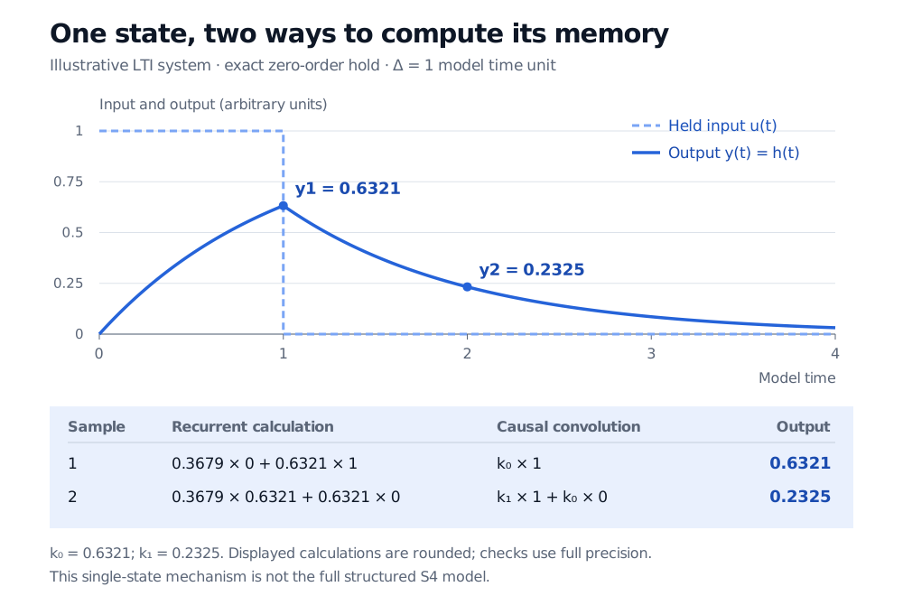
The second output is memory of the first input: nothing new entered during the second interval. The convolution kernel starts with k0=1−e−1 and k1=e−1(1−e−1). Therefore y1=k0u1 and y2=k1u1+k0u2, reproducing both states.
Illustrative scalar system with a unit input held from model time 0 to 1, then zero. Output reaches 0.6321 at time 1 and decays to 0.2325 at time 2. Recurrence and causal convolution produce the same two outputs.
A continuous scalar response sampled once per model time unit. The table compares two representations of the same causal transformation; the system is a teaching example, not a fitted financial model or the full S4 architecture.
This example explains the LTI mechanism. Its single decaying state is not S4’s structured multidimensional memory. It also uses exact zero-order hold; the original S4 paper uses the bilinear discretization rule (§2.3). The numerical coefficients depend on that choice.
What makes S4 structured?
S4 builds on HiPPO memory, which represents input history through polynomial summaries. Its key computational move is a normal-plus-low-rank representation of the state matrix. A unitary change of basis produces diagonal-plus-low-rank form, allowing efficient kernel construction through Cauchy computations rather than repeated dense matrix powers. This is more specific than merely calling a recurrence a state-space model. See the original paper, §§2.2 and 3.
Once the kernel is available, FFT convolution allows parallel computation over a training sequence. Recurrent evaluation carries a fixed-size state as observations arrive. Fixed size means independent of history length, with model dimensions held fixed; it does not mean that an arbitrarily long history is preserved without loss. The official S4 implementation also documents specialised kernels: actual speed depends on the implementation and hardware.
Boundaries that matter in financial use
Mamba makes selected coefficients depend on the input, so one fixed convolution kernel no longer describes the whole sequence. Its selective scan addresses a different computation problem (Gu and Dao, §§3.2–3.3).
A statistical state-space model with a Kalman filter instead specifies a probabilistic latent process and updates uncertainty from noisy observations. An S4 hidden state is not automatically an estimated hedge ratio, posterior distribution or calibrated uncertainty measure.
For forecasting, a causal kernel still requires features that were genuinely available at prediction time. Parallel training over a recorded sequence does not authorise future observations to enter an earlier prediction. Guard against look-ahead bias in preprocessing as well as in the model.