Mamba uses input-dependent state-space updates to select what a sequence model retains. A scalar example explains selective step sizes and their limits.
Mamba selective state-space model
Mamba is a neural sequence architecture built around a selective state-space model: the current input helps determine what enters memory, what persists and what is read out. For a quant processing long streams of order-book events or financial text, the attraction is a compact learned memory that can respond differently to different observations.
This article describes the original Mamba architecture introduced by Gu and Dao in 2023. The official implementation distinguishes its selective SSM layer, the surrounding Mamba block and later Mamba-2 blocks.
Selection changes the memory update
A schematic discrete SSM writes
ht=Atht−1+Btxt,yt=Ctht.
Here xt is the input, ht the hidden state and yt the output. In the original selective layer, Bt, Ct and a positive discretization step Δt depend on the input; the learned continuous state matrix A is shared across positions. Discretization produces At and Bt. Input-dependent coefficients make the overall mapping nonlinear even though each state update has a linear form once those coefficients are fixed. See Gu and Dao, §§2–3.2.
This differs from attention, which forms weighted interactions with other sequence positions. The original Mamba block wraps the selective recurrence with projections, a local causal convolution and gating; its memory mechanism does not require attention. The official repository exposes the block separately from the SSM operation.
A step size can behave like a retention gate
Consider a deliberately simplified scalar system, with the input held constant over one interval:
dτdh=−h+x.
Multiplying by eτ and integrating over an interval of length Δ gives the exact update
hnew=e−Δhprevious+(1−e−Δ)x.
The two weights sum to one. A small positive step preserves most of the previous state; a larger step moves it further toward the current input. This illustrates the connection between discretization and gating discussed in Gu and Dao, §3.5.
Take the previous state as 1 and the held input as 3, in arbitrary units. Compare two alternative single updates:
Model step
Old-state weight
Input weight
New state
Δ=ln2
1/2
1/2
2
Δ=ln4
1/4
3/4
2.5
For the second row, the calculation is 41×1+43×3=2.5. Both updates start from 1; the second is not applied after the first.
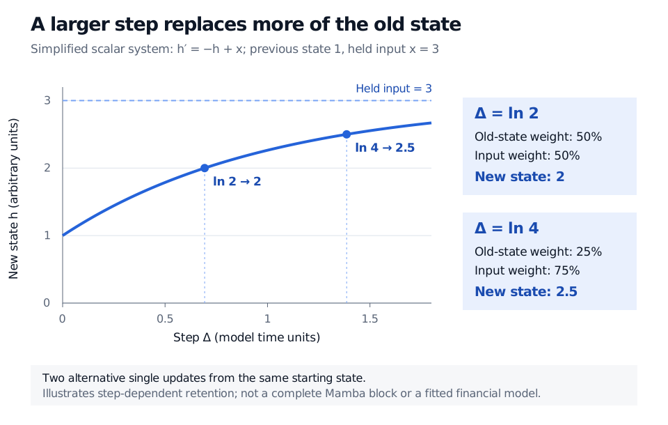
Simplified scalar update from state 1 toward held input 3. At a step of ln 2, old-state retention is 50% and the new state is 2. At ln 4, retention is 25% and the new state is 2.5. These are alternative single updates, not successive steps.
Exact response of the illustrative scalar system. The model step controls the balance between retaining the old state and incorporating the held input; it is not an observed market time interval.
The step is a learned model quantity, not necessarily elapsed seconds or the sampling interval of market data. The example fixes the input coefficient and omits input-dependent readout, multiple channels and the surrounding neural block. It explains selective retention; it is neither a literal implementation of the full original Mamba block nor evidence of forecasting skill.
Why the scan matters
Input-dependent updates prevent the selective layer from using one fixed convolution kernel across the sequence. Mamba instead uses a hardware-aware parallel scan, with fused operations and recomputation to reduce memory traffic. See Gu and Dao, §3.3.
Holding state size, width and depth fixed, recurrent work grows linearly with sequence length. During autoregressive inference, the carried state has fixed size rather than growing with the number of past positions. Training still processes and stores sequence-dependent quantities. Actual speed depends on hardware, kernels, precision and workload; linear scaling alone does not establish a speed advantage for a particular dataset.
For a trading forecast, a causal recurrence only restricts information flow inside the model. Features must also respect their real availability times: revised macro releases, future-normalized inputs or labels leaking into preprocessing can introduce look-ahead bias before the recurrence begins. Compare models on the same chronological splits, prediction horizon and execution assumptions. Efficiently retaining a long history does not guarantee that the retained information predicts future returns.
To compare this retention mechanism with other learned memory gates, read the SelfMadeQuant lesson Gated Memory: LSTMs and GRUs (public preview; full lesson requires membership).