Snapshot ensembles average predictions from saved states of one cyclic training run. See why probability averaging differs from averaging logits or weights.
Snapshot ensemble
A snapshot ensemble combines predictions from several saved states of one neural network trained along a cyclic learning-rate trajectory. A quant researcher can obtain several forecast models within one training run, then average their outputs. The saved models share their training history; they do not provide independent evidence about future markets.
Save at the quiet end of each cycle
The method introduced by Huang and colleagues repeatedly lowers the learning rate, saves a model near the end of a cycle, then raises the rate to encourage further exploration. Its aim is to collect models that predict well but make different errors, rather than save every intermediate training state.
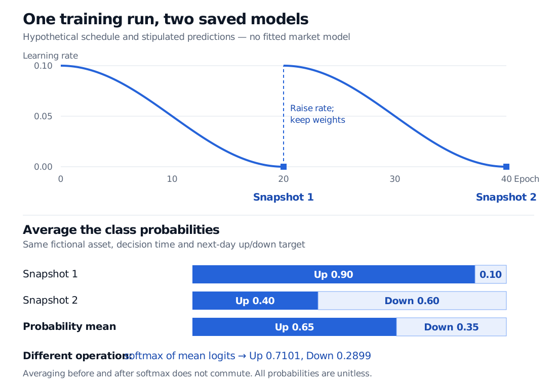
The learning-rate schedule controls the size of parameter updates. In the cosine schedule used by the original method, each cycle moves from a large rate towards a small one. A restart raises the rate while continuing from the current weights: it does not randomly initialise a fresh network. This is the warm-restart mechanism described in SGDR, §3. A new cycle can temporarily worsen predictions, and another cycle need not find a distinct or better solution.
At prediction time, load each retained snapshot, evaluate it on the same input and combine its output. For classification, the original snapshot-ensemble rule averages the models' softmax probabilities. For a retained set of m snapshots,
pˉ(c∣x)=m1j=1∑mp(c∣x;θj),
where c is a class, x is the common input and θj identifies snapshot j. The paper ensembles the last m snapshots; that historical convention is not a guarantee that later snapshots are best on a new task. See Huang et al., §3.
A hypothetical two-cycle learning-rate schedule saves models at epochs 20 and 40 without resetting weights. Stipulated up/down probabilities 0.90/0.10 and 0.40/0.60 average to 0.65/0.35. Softmax of mean logits instead gives approximately 0.7101/0.2899.
Original hypothetical schedule and stipulated predictions. The curve shows learning rate, not training loss or measured model quality; probabilities are unitless.
Probability averaging is a particular operation
Suppose two saved models classify the same fictional asset's next-day return as up or down, with identical class definitions and information cutoff:
Saved model
Up
Down
Snapshot 1
0.90
0.10
Snapshot 2
0.40
0.60
Equal probability average
0.65
0.35
The average assigns 0.65 to up because (0.90+0.40)/2=0.65. There is no realised outcome in this example, so it establishes neither accuracy nor probability calibration.
Averaging the logits first gives a different answer. At temperature 1, logits (ln9,0) produce the first row and (0,ln1.5) produce the second. Their mean logits give up probability
That is a valid calculation of a different aggregation rule. Softmax is nonlinear, so “average then softmax” cannot silently replace “softmax then average.” A vote over the two winning class labels would be yet another rule, producing a tie here.
Three operations that can be confused
Operation
What is retained and used for inference?
Select one best checkpoint
One model, selected using a declared validation criterion
Snapshot ensemble
Several saved models, whose predictions are combined
Stochastic weight averaging
One model formed by averaging suitable parameter vectors
Stochastic weight averaging averages in parameter space. It therefore need not reproduce an average of model predictions. The SWA paper, §§3.2–3.3 describes its single-model inference advantage and the need to update batch-normalisation statistics where applicable. Keeping arbitrary checkpoints or averaging arbitrary weights is not interchangeable with either named method.
The saving has boundaries
The original “train one” comparison concerns a fixed training budget, rather than separately training every ensemble member from scratch. It does not remove snapshot storage or the work of evaluating several models. Searching schedules and running validation also consume compute. Save the state needed to reproduce inference, including relevant normalisation buffers and preprocessing, not just a list of epoch numbers.
For financial research, cycle lengths, retained snapshots and any ensemble weights are model-selection choices. Choose them within the development data, then evaluate the frozen procedure on later held-out observations. Each historical refit must use only features and completed labels available at its cutoff. The Time-Ordered Train, Validation and Test Design lesson develops this separation; its preview is public and the full lesson requires membership.
Snapshots from one trajectory can remain highly dependent. They are neither independent training runs nor independent, identically distributed posterior samples. Disagreement between them is not, by itself, a calibrated uncertainty interval. If all snapshots inherit the same leaked feature, regime failure or systematic forecasting error, averaging preserves that problem. Test accuracy, calibration and economic usefulness separately; none is guaranteed by the averaging rule.