Siamese network: Definition & Examples

A Siamese network compares two inputs by passing each through the same neural network, with one shared set of parameters, and comparing the resulting representations. For a quant matching financial disclosures, the useful question is whether two passages describe the same kind of event despite different wording. The network supplies a comparison score; its training pairs define what “same kind” means.

The classical architecture appeared in Bromley and co-authors’ signature-verification work. Two branches extract features using identical weights. Sharing is the defining constraint: two separately trained encoders with the same layer shapes are not the classical Siamese construction.

Two inputs, one learned rule

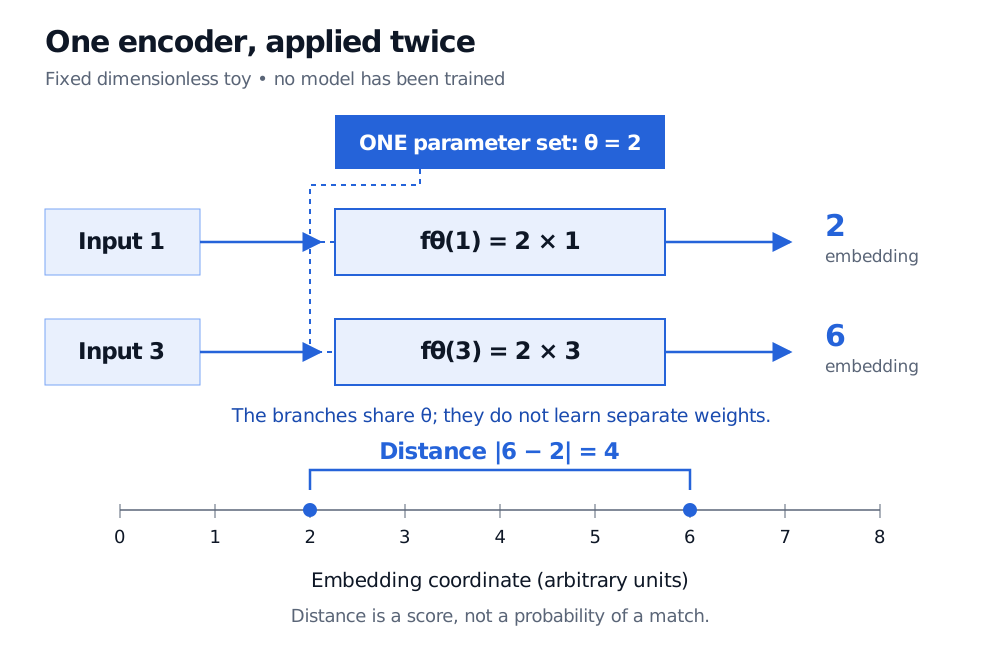
Write the encoder as $f_\theta$ , where $\theta$ is its single parameter set. For inputs $\mathbf{x}_1$ and $\mathbf{x}_2$ , an example comparison is Euclidean distance:

D_\theta(\mathbf{x}_1,\mathbf{x}_2) =\lVert f_\theta(\mathbf{x}_1)-f_\theta(\mathbf{x}_2)\rVert_2.

The encoder produces an embedding, a vector representing each input. The shared map and this symmetric distance make swapping the inputs leave the score unchanged. Chopra, Hadsell and LeCun describe learning such a representation for verification, including comparisons involving identities absent from training. That capability is an evaluation objective, not a guarantee for every new identity.

The architecture can support metric learning, but it is not itself a loss function. Nor does every contrastive-learning method require a classical Siamese pair of branches.

Consider the smallest possible calculation: a fixed scalar encoder,

f_\theta(x)=2x

, with dimensionless inputs 1 and 3. It produces embeddings 2 and 6, so

D_\theta(1,3)=\lvert 2-6\rvert=4.

The multiplier 2 is applied twice; there are no separate left and right multipliers. This toy demonstrates parameter sharing and distance computation. It has learned no semantic meaning, and 4 has no universal interpretation as “similar” or “different.”

Fixed dimensionless example: one shared parameter theta equals 2 maps input 1 to embedding 2 and input 3 to embedding 6. Their Euclidean distance is 4 arbitrary embedding units.

One parameter set serves both branches. The distance is 4 embedding units, not a probability of a match.

What the training pairs ask it to preserve

One possible objective is the contrastive loss used by Hadsell, Chopra and LeCun. With the convention $Y=0$ for similar pairs and $Y=1$ for dissimilar pairs, and margin

m>0

L(\theta)=\frac{1-Y}{2}D_\theta^2 +\frac{Y}{2}\max(0,m-D_\theta)^2.

Similar pairs are penalised for being apart. Dissimilar pairs are penalised only inside the margin. Their paper describes summing the gradient contributions from both branches to update the shared parameters. Labels in other implementations may reverse this convention; check the loss before assigning them.

For the fixed toy distance 4 and an illustrative margin 5, the loss would be 8 if the pair were labelled similar, or 0.5 if labelled dissimilar. These are alternative labels for the same calculation, not simultaneous training labels. This loss alone does not require dissimilar distances to grow indefinitely. Training only by bringing similar pairs together admits collapse: a constant encoder puts every input at the same point.

In a disclosure-matching application, positive pairs might be independently labelled descriptions of the same event type. Negative pairs should include plausible confusions, such as two passages sharing accounting vocabulary but describing different events. This is a proposed research use: shared weights do not establish that the labels capture an economically useful distinction.

The owned Embeddings lesson develops representation choices and why a convincing vector analogy is insufficient evidence for a financial-text task. A public preview is available; the full lesson requires membership.

Split the underlying records before making pairs

A held-out pair can still contain a document already used in training, or a near duplicate of it. Randomly splitting a prebuilt pair table can therefore test familiarity with its components. Separate underlying records first, then construct training pairs within the training partition. If the claim concerns unseen issuers or identities, keep those groups separate too; allowing the same issuer in both periods answers a different generalisation question.

For a historical research test, also respect chronology and availability. An embedding fitted on later disclosures or pair labels derived from outcomes not yet observed can create look-ahead bias. Fit preprocessing and encoder parameters on training data, choose the distance threshold on validation data, and leave the final test data untouched. This applies the scikit-learn leakage guidance to the components of a pair model.

Finally, evaluate the intended decision. A small distance is a comparison under the fitted representation. It is not automatically a calibrated probability, proof that two events have the same economic consequences, or evidence of a profitable signal.

Sources

Jane Bromley and co-authors, “Signature Verification Using a ‘Siamese’ Time Delay Neural Network” (1993), §4: paired branches constrained to identical weights.
Sumit Chopra, Raia Hadsell and Yann LeCun, “Learning a Similarity Metric Discriminatively, with Application to Face Verification” (2005), §§1–2: shared mapping, symmetric comparison and verification for previously unseen identities.
Raia Hadsell, Sumit Chopra and Yann LeCun, “Dimensionality Reduction by Learning an Invariant Mapping” (CVPR 2006; author manuscript dated November 2005), §§2.1 and 3.1: contrastive-loss labels, margin, collapse and shared-parameter training.
scikit-learn, “Common pitfalls and recommended practices”, §§12.1–12.2: consistent preprocessing, splitting first and training-only fitting.

Two inputs, one learned rule

What the training pairs ask it to preserve

Split the underlying records before making pairs

Sources

Related terms

Look-ahead bias

Metric learning

Neural network