Learn a task-specific distance from labels, pairs or triplets; connect a positive semidefinite matrix to a linear map and avoid leakage in financial validation.
Metric learning
Metric learning estimates a distance function from data so that closeness reflects a chosen learning task. For a quant retrieving comparable historical market states, this makes the meaning of “comparable” part of the fitted model. A distance trained to recognise liquidity conditions can differ from one trained to recognise volatility conditions, even on the same features.
In supervised metric learning, the training signal can be class labels, pairs marked similar or dissimilar, or triplets saying “this observation should be closer to that one than to the other.” Selecting a distance matrix by hand specifies a geometry; fitting its parameters against such evidence is the learning step. Xing and co-authors develop the pair-based approach.
What teaches the distance?
Consider training records with market-state labels. A k-nearest neighbors classifier can use a learned distance to choose which historical labels vote on a new state. Large margin nearest neighbor learning, LMNN, pulls selected same-class target neighbors closer while penalising differently labelled records that enter their margin. It does not require every record of a class to collapse into one cluster. These are training objectives, with no guarantee of correct classification on unseen data. Weinberger and Saul, §§3.1–3.2 describe this construction.
The definition of similarity matters. Sector labels teach a different comparison from labels based on subsequent returns. Merely minimising distances between similar pairs has a useless solution: map everything to the same point. Dissimilarity constraints or a competing separation objective prevent that particular collapse, as in Xing and co-authors’ formulation. No algorithm supplies the economically appropriate labels automatically.
If M=L⊤L, this is ordinary Euclidean distance after applying the same linear map to both points:
dM(x,y)=∥Lx−Ly∥2.
This is often called a learned Mahalanobis distance, although its matrix need not be an inverse sample covariance. Here the weights are fitted to the learning objective. The squared distance is convenient in losses, but the square root above is needed for the usual metric triangle inequality.
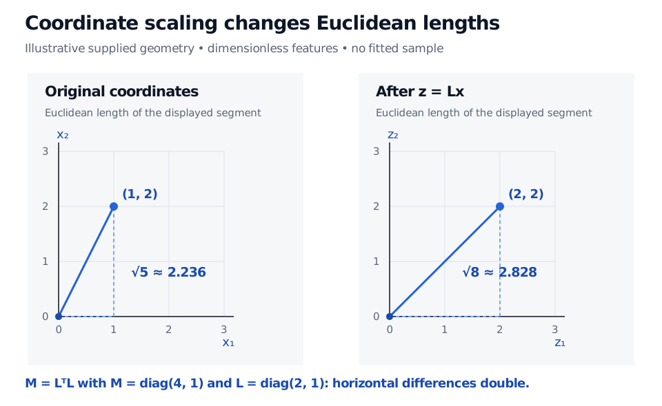
For an illustrative supplied result, suppose dimensionless features have displacement (1,2)⊤ and
Transforming the displacement gives (2,2)⊤, whose length is also 8. The first coordinate receives four times the weight in the squared distance, corresponding to twice the coordinate scale. These numbers demonstrate the geometry; no training sample was fitted to obtain this matrix.
Illustrative dimensionless geometry. Original displacement (1, 2) has Euclidean length square root 5, approximately 2.236. Transforming with L diagonal (2, 1) gives displacement (2, 2), with length square root 8, approximately 2.828.
An illustrative supplied matrix doubles horizontal differences through L. Euclidean length after transformation equals the learned distance before transformation; it need not equal the original Euclidean length.
Positive semidefiniteness permits zero eigenvalues. With M=diag(1,0), the distinct points (0,0)⊤ and (0,1)⊤ have distance zero: the second direction is discarded. This is a pseudometric on the original space. Positive definiteness is needed to distinguish every pair of distinct input vectors across the full space. The distinction is explicit in Weinberger and Saul’s §2.1.
Positive Definite Matrices develops these quadratic-form and factorisation foundations. The full lesson requires membership; a public preview is available.
Keep the learned geometry inside the training split
Treat scaling, construction of training pairs or triplets, and metric fitting as parts of model training. Within each validation fold, fit them using that fold’s training records; apply the resulting fixed transformation to its validation records. Use validation to choose settings, then reserve an untouched test period for final evaluation. The scikit-learn leakage guidance explains why fitting transformations before splitting contaminates evaluation.
For historical market-state retrieval, each training label must already be observable at the simulated prediction time. A label defined by a later return cannot enter training until its outcome horizon has elapsed. Constructing pairs across the evaluation boundary can expose those outcomes even if the final classifier itself only sees training rows.
A smaller distance establishes similarity under the fitted representation. It establishes neither a causal link between features and outcomes nor a profitable trading rule. Check performance on the intended held-out task: a geometry that fits one notion of similarity may be unsuitable for another.